Abstract
As part of a research project, I contributed to the development and testing of a Visual Servoing framework, a control strategy that links image feature variations to robot velocities. Applied to autonomous vehicles, this approach enables lane-keeping purely from camera input, without GPS or map dependency. It integrates lane detection using deep learning and transforms the output into features used in a control law that centers the vehicle in the lane.
The system was validated on simulated and real data, showing robust behavior in diverse road scenarios.
Visual Servoing Concepts
Visual Servoing (VS) refers to the use of visual information, typically from a camera, to control the motion of a robot. The control law is derived from the error between a current image feature $s$ and a desired one $s^*$:
$$ e(t) = s(t) - s^* \quad \text{Eq (1)} $$
The relationship between the change in feature and the robot velocity $u_c$ is modeled by the interaction matrix $L_s$:
$$ \dot{s}(t) = L_s u_c \quad \text{Eq (2)} $$
To ensure convergence, exponential decay is applied to the error:
$$ \dot{e}(t) = -\lambda L_s^+ e(t) \quad \text{Eq (3)} $$
Where $L_s^+$ is the Moore–Penrose pseudo-inverse of $L_s$.
Feature Extraction from Camera Image
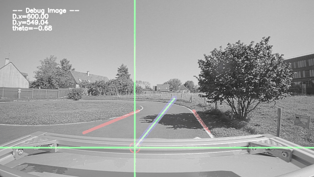
The visual servoing controller relies on three geometric features computed from the lane detection in the image:
- $X$: lateral offset between the image center and a selected target point on the lane
- $Y$: vertical position (depth proxy) of the point in the image
- $\Theta$: angular deviation between the lane direction and the vertical image axis
These features are extracted in the image frame and used as input for control.
Selection of Target Point
The detected lane is assumed to provide a centerline defined as a curve in image space. A single target point is selected at a fixed vertical distance from the bottom of the image (typically 3/4 of the image height), denoted $v_t$.
The horizontal position of this point is obtained by evaluating the lane curve at $v_t$:
$$ u_t = f(v_t) \quad \text{Eq (4)} $$
Where $f$ is the polynomial fitted to the detected centerline.
Computation of X and Y
The coordinates $(u_t, v_t)$ are image pixel coordinates. They are normalized relative to the optical center $(c_x, c_y)$ and focal lengths $(f_x, f_y)$:
$$ X = \frac{u_t - c_x}{f_x}, \quad Y = \frac{v_t - c_y}{f_y} \quad \text{Eq (5)} $$
$X$ corresponds to the lateral displacement in the image, and $Y$ is a proxy for depth.
Estimation of Theta
To compute the orientation of the lane at the target point, the tangent to the fitted curve is calculated:
$$ \Theta = \arctan\left( \frac{df}{dv}(v_t) \right) \quad \text{Eq (6)} $$
This angle represents the deviation between the lane direction and the vertical axis of the image.
Final Feature Vector
The visual features used in control are then assembled as:
$$ s = [X, Y, \Theta]^T \quad \text{Eq (7)} $$
This vector $s$ is compared to a desired reference $s^*$ to compute the control error.
Lane Detection via Deep Learning
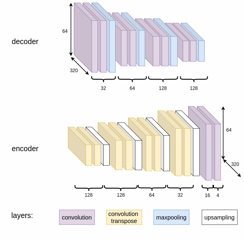
The first step in feature extraction is robust lane detection. Instead of relying on geometric models, which are brittle in poor lighting or degraded markings, a convolutional autoencoder trained on the CULane dataset is employed.
The model produces binary segmentation maps for lane positions, which are then used to compute the path to follow.
From Feature to Control
Velocity Computation
Given the extracted features $s = [X, Y, \Theta]$, the control goal is to minimize the error $e = s - s^*$. The control output $u_r = [v, w]^T$ includes linear and angular velocity commands.
The time derivative of the features is related to the robot velocity by:
$$ \dot{s} = L_s(X, Y, \Theta) C_{TR} u_r \quad \text{Eq (8)} $$
Where $C_{TR}$ is the transformation matrix between robot and camera frames.
Control Law
Two control configurations are used depending on the desired feature.
When the vehicle is far from the lane, the feature point appears above the image bottom, requiring the column controller to guide the vehicle back.
When the feature point remains near the bottom of the image, the row controller is used to maintain lane position.
Row controller for $s^* = [0, Y, 0]$:
$$ w = -B_{row}^+ \left( \begin{bmatrix} K_X e_X \\ K_\Theta e_\Theta \end{bmatrix} + A_{row} v_d \right) \quad \text{Eq (9)} $$
Column controller for $s^* = [X, 0, \pm \frac{\pi}{4}]$:
$$ w = -B_{col}^+ \left( \begin{bmatrix} K_Y e_Y \\ K_\Theta e_\Theta \end{bmatrix} + A_{col} v_d \right) \quad \text{Eq (10)} $$
Where $v_d$ is the desired forward velocity and the matrices $A$ and $B$ are derived from the interaction matrix and transformation.
Control in Real-Time
The computed velocities are sent to the vehicle’s motion controller. The system operates in real time and does not depend on external GPS or map input, ensuring portability and robustness in unmapped environments.
Integration into the Dynamic Window Approach (DWA)
The Visual Servoing framework can be integrated into a classical Dynamic Window Approach (DWA) by modifying the objective function. Rather than relying solely on geometric terms like heading angle or distance to a local goal, the Visual Servoing error is incorporated as part of the scoring function.
Goal Function
Each motion command candidate $(v, w)$ generated by the DWA is evaluated not only for obstacle avoidance and kinematic feasibility, but also based on how well it aligns the robot with the desired image-based features.
$$ J_{vs}(v, w) = \| s(v, w) - s^* \| \quad \text{Eq (11)} $$
This VS-based cost is added to the standard DWA cost terms:
$$ J_{\text{total}} = \alpha J_{\text{obs}} + \beta J_{\text{vel}} + \gamma J_{vs} \quad \text{Eq (12)} $$
Where:
- $J_{\text{obs}}$ evaluates obstacle clearance
- $J_{\text{vel}}$ encourages high velocity
- $J_{vs}$ penalizes deviation from visual servoing objectives
- $\alpha$, $\beta$, $\gamma$ are tunable gains
Obstacle Function
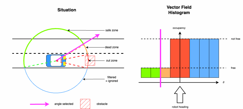
As explained in the project Optimization Of The Dynamic Window Approach (DWA), the obstacle avoidance function requires a safety angle to be determined.
The following figure illustrates the computation of this angle. The angle must satisfy constraints to:
- avoid collisions;
- maintain a safe distance from obstacles;
- remain within navigable space.
The last constraint is critical, as omitting it could result in the vehicle leaving the road.
Results
By integrating $J_{vs}$, the DWA selects trajectories that are not only dynamically valid and safe, but also visually consistent with the lane-following objective defined by the Visual Servoing framework.