Abstract
A multimodal deep learning model was developed to predict human driving behavior over a short time horizon. The training dataset was recorded specifically for this project.
More details about this work are provided in PredictionPousseur 2022 .
Introduction
Driving intention is represented as a sequence of vehicle states. Let $I$ be:
$$ I = \{x_0, x_1, ..., x_n\} \quad \text{Eq (1)} $$
Here, $(x_i) = (v_i, w_i)$ denotes the state at time $i$, where $v_i$ is the linear velocity and $w_i$ is the angular velocity.
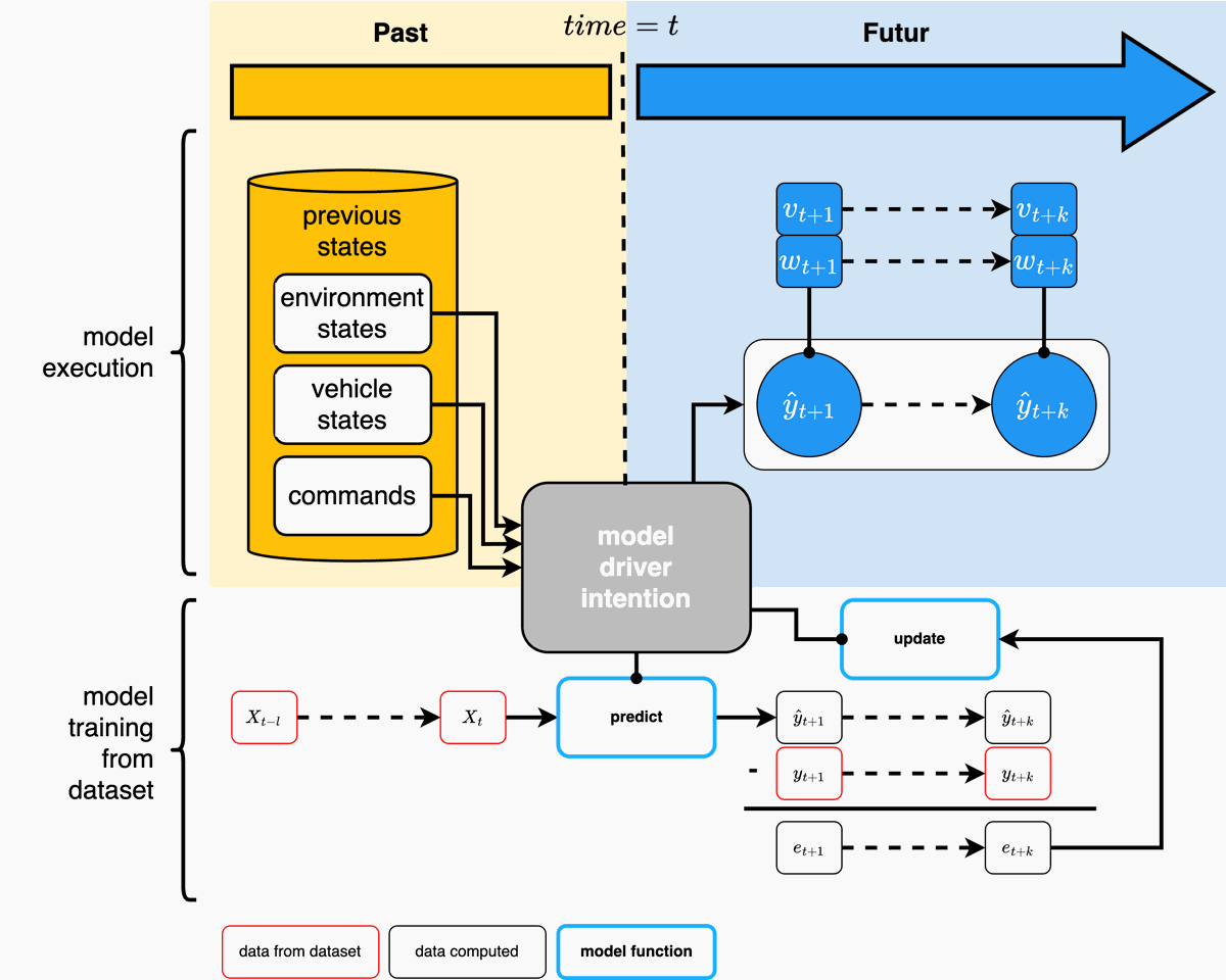
The prediction model, $H_\Theta$, aims to produce:
$$ H_\Theta(X) = \{\hat{y}_{t+1},...,\hat{y}_{t+k}\} \quad \text{Eq (2)} $$
where
- $ \Theta $ are the model parameters, $ X $ is the input vector at time $ t $
- $ \hat{y}_{t+i} $ is the predicted state
- $ (v_{t+i}, w_{t+i}) $ are the predicted velocities
- $ dt $ is the acquisition interval in seconds.
Data and Model
Data Categories
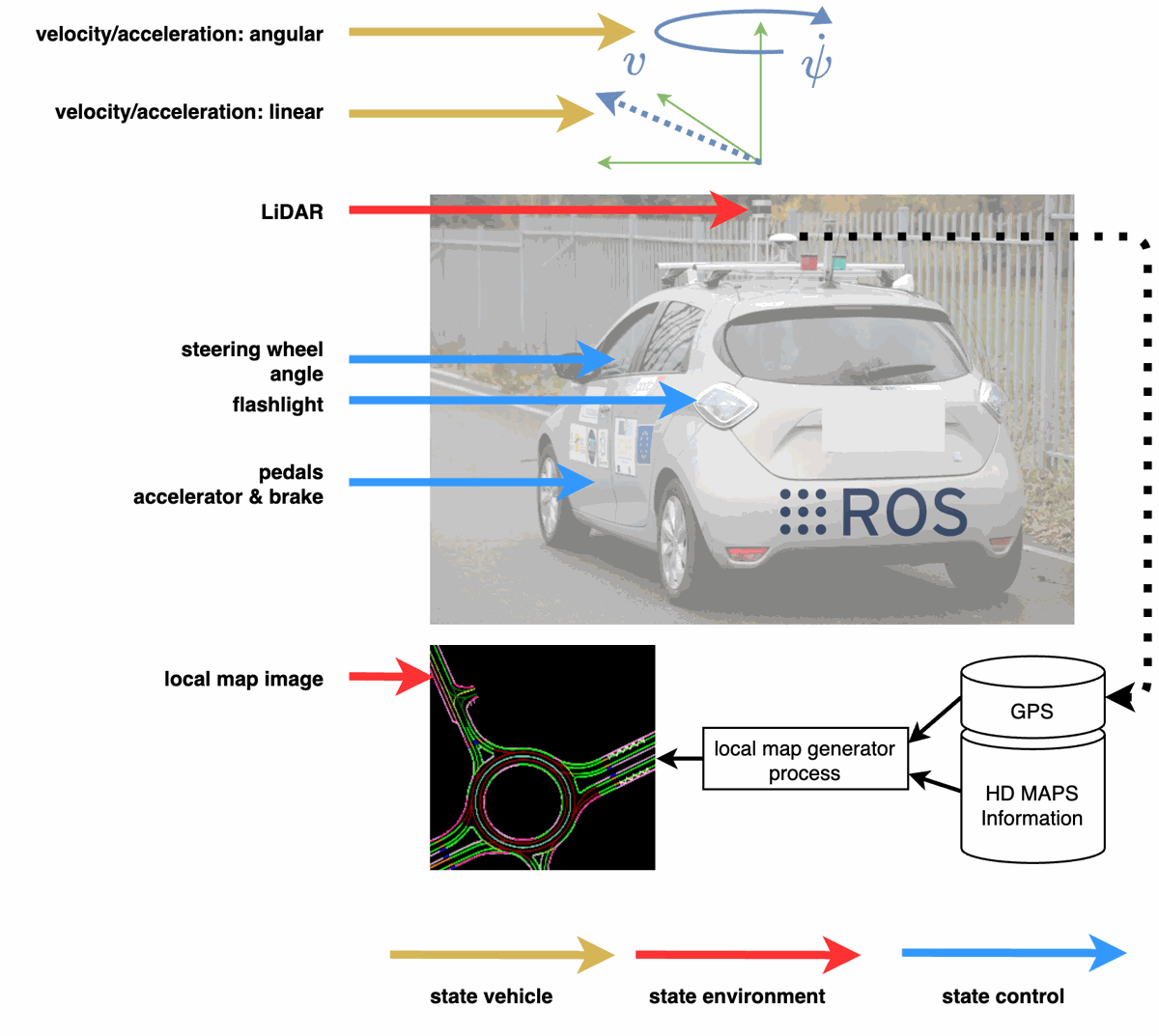
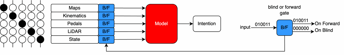
Input data are grouped into three categories:
- Vehicle state: velocities, accelerations, and other dynamics.
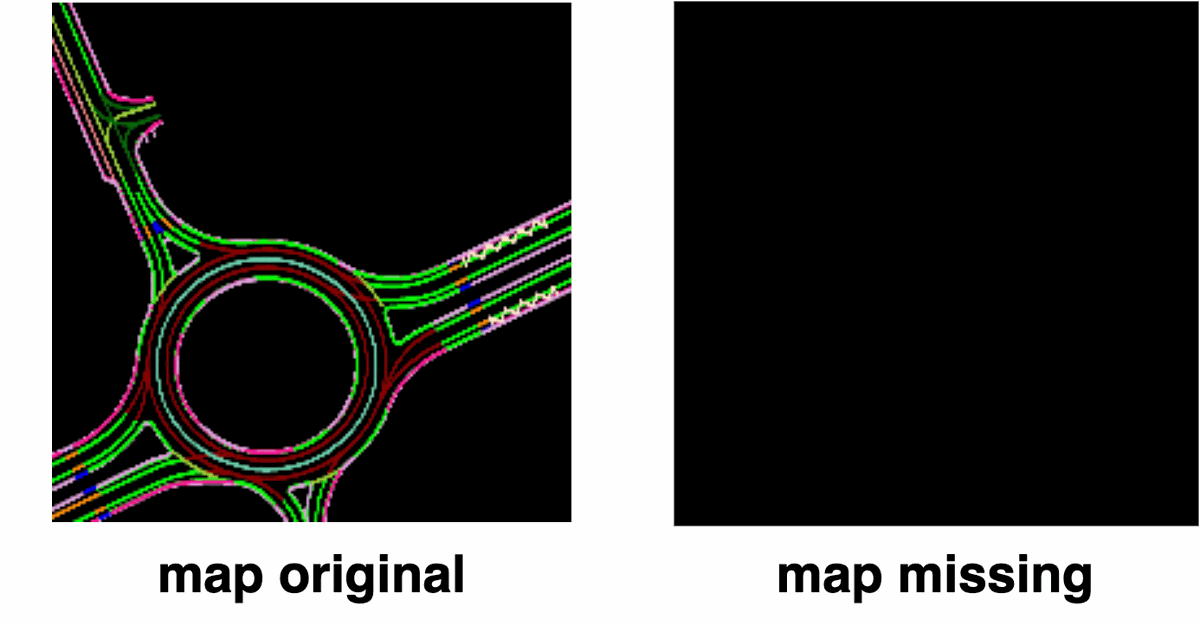
- Environment state: map and Lidar data.
- Control state: steering angle, pedal positions.
Driving Scenarios
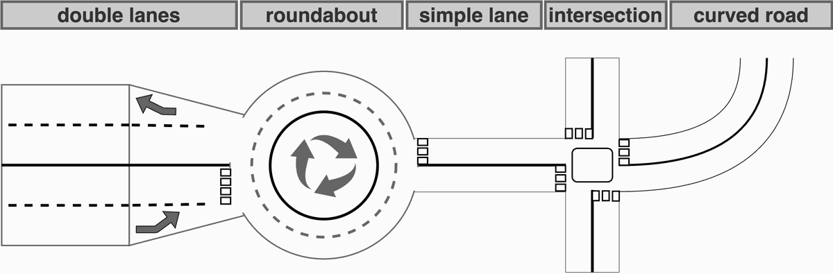
Behavior varies across scenarios such as highways, city streets, and roundabouts. The dataset includes both structured (lane-marked roads) and unstructured (urban intersections, roundabouts) environments to prevent bias.
Temporal Aspects
No manual labeling was required; future velocities served as output targets. The sensor acquisition rate is $dt = 100ms$ (10 Hz). A sliding window over past states captures temporal dependencies, and data augmentation (time warping, resampling) improves generalization.
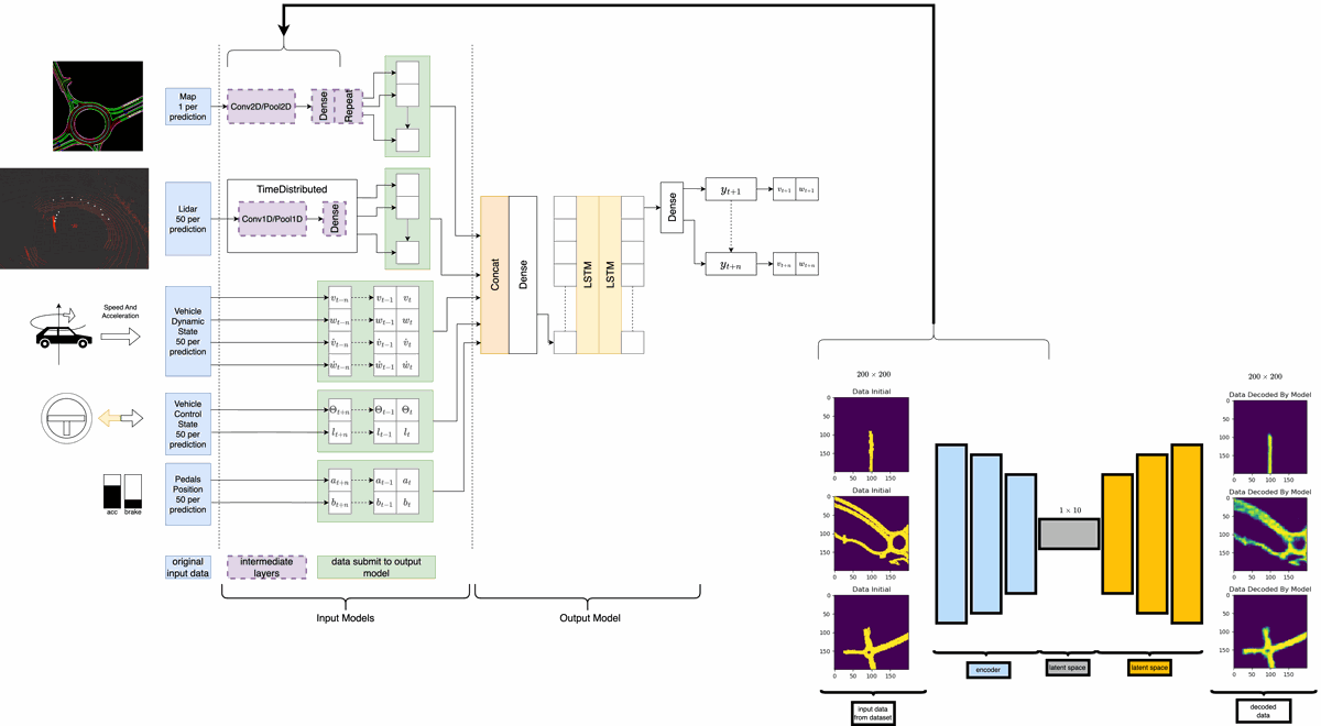
Multi-Modal Model
The model consists of:
- Input model: compresses each modality into a latent vector.
- Final model: concatenates latent vectors and applies a recurrent network.
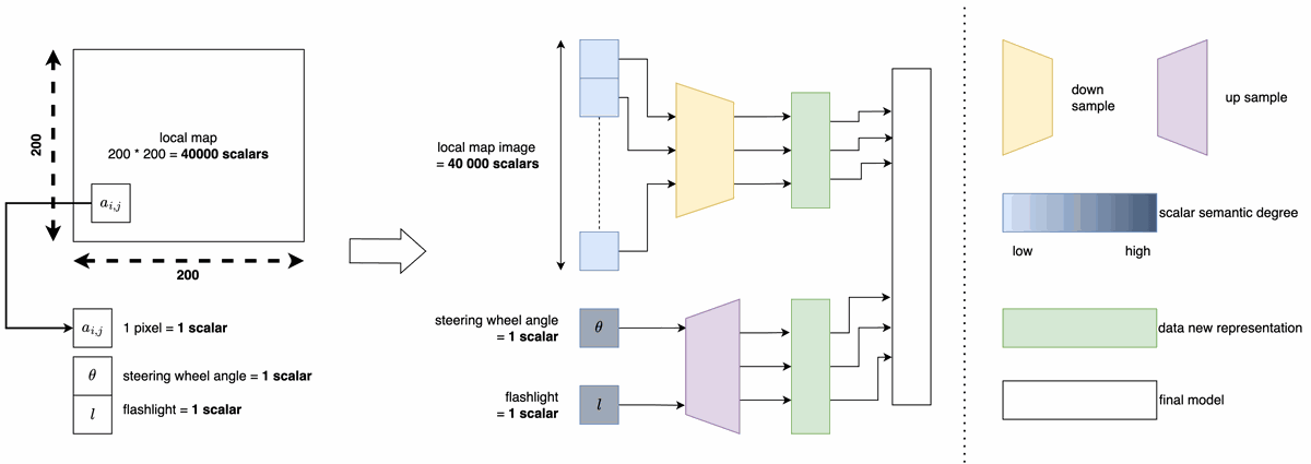
The input model uses:
- CNNs for image-based features (camera, Lidar projections).
- Fully connected layers for numerical data.
The final model uses GRUs for sequence prediction.
Results
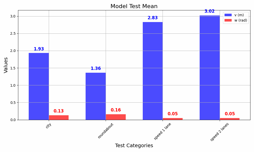
Test Characteristics
| Test Name | Roundabouts | Intersections | Speed Limit | Distance | Time Record | Lanes |
|---|---|---|---|---|---|---|
| roundabout | 6 | 1 | 70 km/h | 4 km | 378 s | 2 |
| city | 4 | 7 | 50 km/h | 4 km | 519 s | 1 |
| speed (1 lane) | 2 | 0 | 70 km/h | 2 km | 116 s | 1 |
| speed (2 lanes) | 0 | 0 | 90 km/h | 2 km | 84 s | 2 |
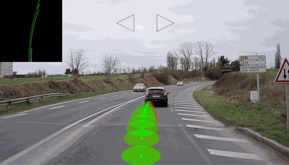
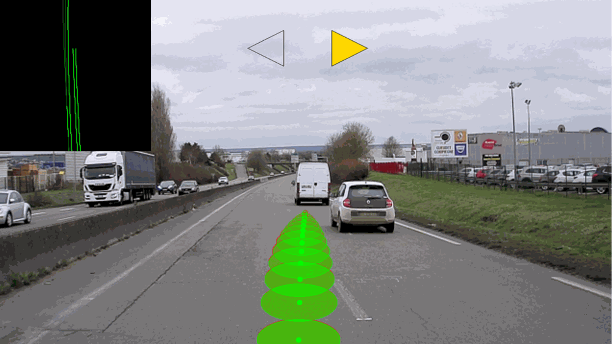
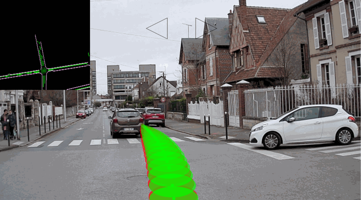
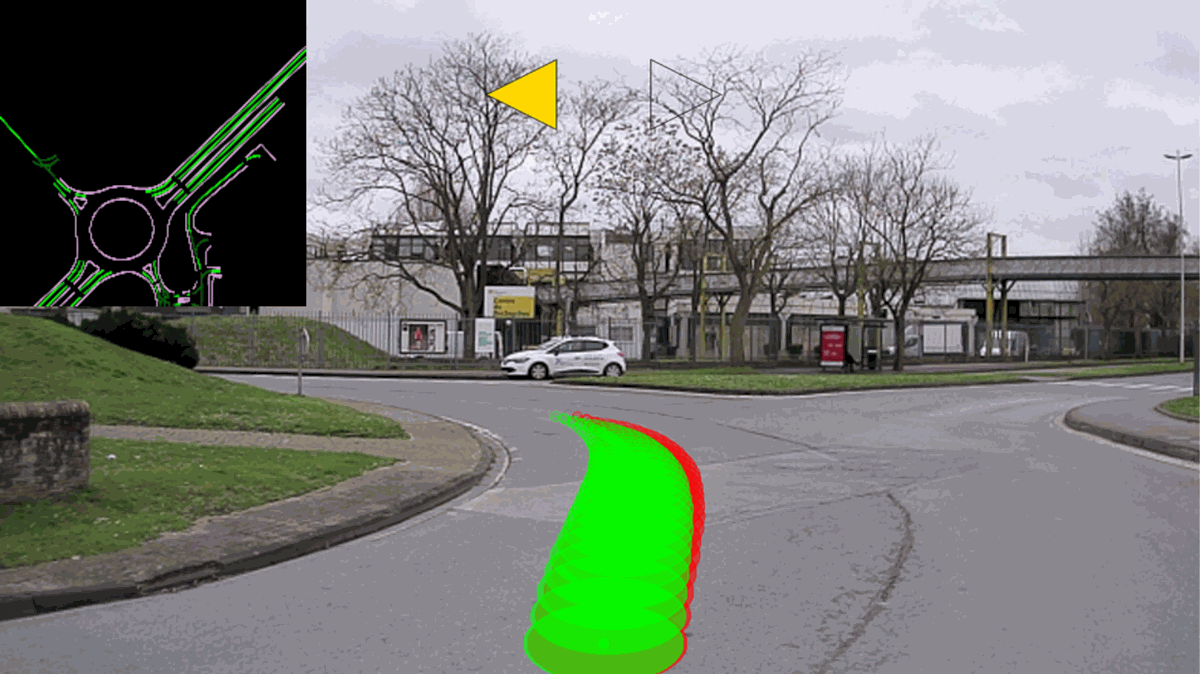
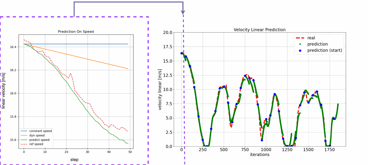
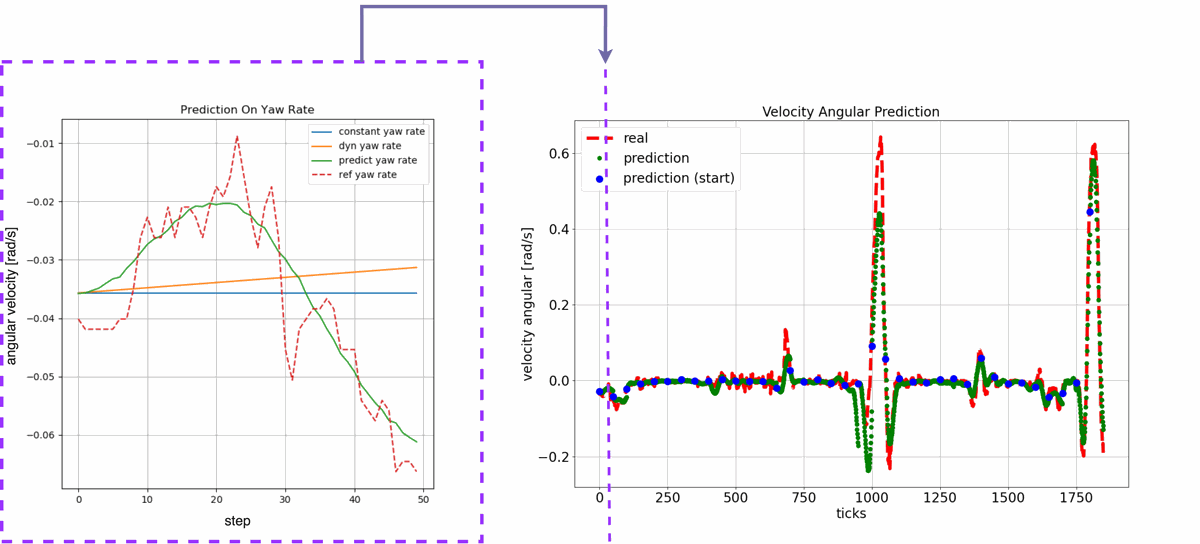
The following projections compare predicted and actual trajectories for different scenarios.
The error function is:
$$ loss(y_{predict},y_{true}) = w_{v} \cdot \sum_{i=0}^{n} | y_{predict,v,i} - y_{true,v,i} | + w_{w} \cdot \sum_{i=0}^{n} | y_{predict,w,i} - y_{true,w,i} | \quad \text{Eq (3)} $$
Where:
- $w_v$ is the weight for linear velocity error.
- $w_w$ is the weight for angular velocity error.
Example: City Test
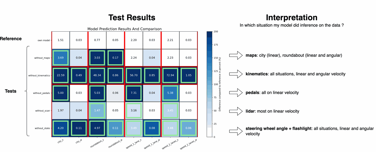
Sensitivity Analysis
The impact of each input was measured by neutralizing it and observing the change in error. This shows which inputs most influence predictions.
References
- Prediction of human driving behavior using deep learning: a recurrent learning structure
Hugo Pousseur, Alessandro Correa Victorino
IEEE ITSC 2022
[Access PDF]