Overview
Source Code
In addition to the main GitHub project, the following submodules are available:
- Dataset of scanned legs (with labels): https://github.com/PouceHeure/dataset_lidar2D_legs
- Labeling GUI tool: https://github.com/PouceHeure/lidar_tool_label
- Radar interface: https://github.com/PouceHeure/ros_pygame_radar_2D
Context
This project detects human legs from 2D LiDAR scans using a Recurrent Neural Network (RNN) with LSTM cells. The LSTM processes each scan as a spatial sequence ordered by angle $ \theta $, not as a time series. The model learns local shape patterns in polar space that are typical of legs.
Pipeline
End-to-end steps:
- Data acquisition with a 2D LiDAR
- Custom labeling and annotation
- Spatial clustering and sequence building
- LSTM training
- Real-time ROS integration and visualization
Demo: Video 1: Video demo: legs detection from a 2D LiDAR scan. .
Input Representation
Each LiDAR scan is a set of polar points:
$$ P_i = (\theta_i, r_i) \quad \text{Eq (1)} $$
where $ \theta_i $ is the angle of point $ i $ (radians) and $ r_i $ is its range (meters).
To form model inputs, points are grouped into clusters using two metrics:
- Polar-plane Euclidean distance
- Radial difference
$$ d_{\text{polar}}(P_i, P_j) = \sqrt{r_i^{2} + r_j^{2} - 2 r_i r_j \cos(\theta_i - \theta_j)} \quad \text{Eq (2)} $$
$$ d_{\text{radius}}(P_i, P_j) = |r_i - r_j| \quad \text{Eq (3)} $$
Two points are connected if both metrics are below thresholds limit_distance and limit_radius. Each connected component (cluster) is encoded as an angle-ordered sequence:
$$ C = \{ P_1, P_2, \dots, P_n \} \quad \text{Eq (4)} $$
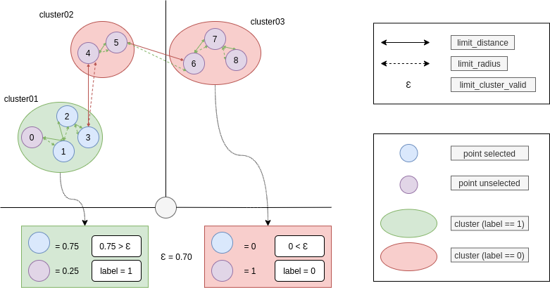
The Fig. 1 defines the variables used to describe each cluster. Each cluster sequence $ C $ is then passed to the LSTM classifier.
LSTM Model
The LSTM captures dependencies along the ordered scan. Typical leg returns form smooth, narrow arcs or symmetric curves. The network relies on:
- Changes in $ r $ along $ \theta $
- Relative angular spacing of points
- Local curvature cues derived from neighboring points
Model Output and Training Loss
The classifier outputs a probability $ \hat{y} \in [0, 1] $ for the class “leg.” A prediction threshold (for example, $0.5$) yields a binary label:
1for leg0otherwise
Training uses binary cross-entropy:
$$ \mathcal{L}_{\text{BCE}} = -\big( y \log(\hat{y}) + (1 - y) \log(1 - \hat{y}) \big) \quad \text{Eq (5)} $$
where $ y \in {0, 1} $ is the ground-truth label and $ \hat{y} $ is the predicted probability.
Estimating the Center of a Detected Cluster
For each cluster $C = \{ P_1, P_2, \dots, P_n \}$ with $ P_i = (\theta_i, r_i) $ that is classified as a leg, the polar center is computed as:
$$ \theta_{\text{center}} = \frac{1}{n} \sum_{i=1}^{n} \theta_i \quad \text{Eq (6)} $$
$$ r_{\text{center}} = \frac{1}{n} \sum_{i=1}^{n} r_i \quad \text{Eq (7)} $$
Here, $ \theta_{\text{center}} $ is the mean angular position and $ r_{\text{center}} $ is the mean range of the cluster, with $ n $ the number of points. The polar center can be converted to Cartesian coordinates:
$$ x = r_{\text{center}} \cos(\theta_{\text{center}}), \quad y = r_{\text{center}} \sin(\theta_{\text{center}}) \quad \text{Eq (8)} $$
These estimates are used during evaluation and in real-time ROS inference.
Training and Augmentation
Positive clusters are augmented by rotation to improve generalization:
$$ \theta_i' = \theta_i + \Delta \theta \quad \text{Eq (9)} $$
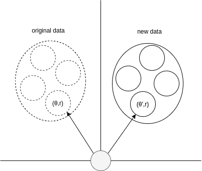
The Fig. 2 shows how rotation preserves a cluster’s internal structure while changing its orientation.
To address class imbalance, positives are upsampled. The final dataset size is:
$$ \text{Final dataset size} = N + K \cdot N_{\text{positive}} \quad \text{Eq (10)} $$
where $ N $ is the original dataset size, $ N_{\text{positive}} $ the number of positive clusters, and $ K $ the number of augmentation steps.
Training curves:
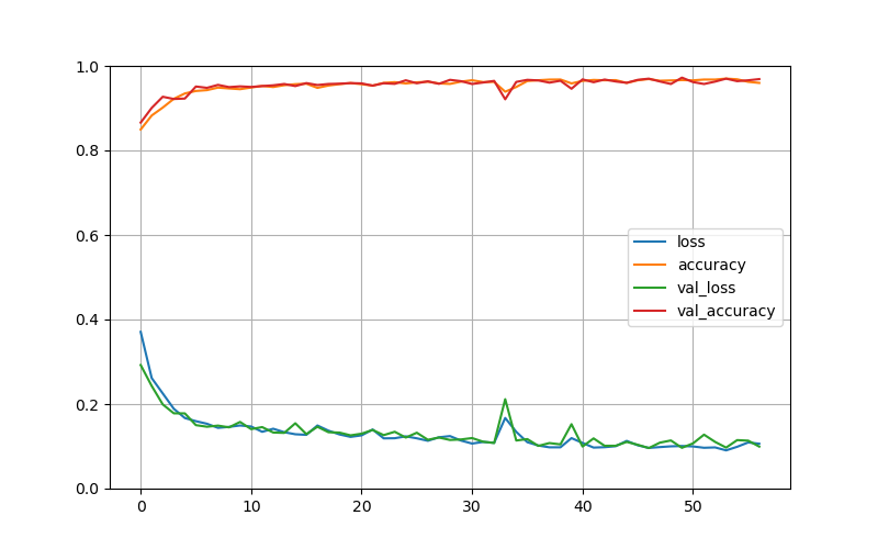
The Fig. 3 summarizes optimization progress and generalization metrics.
Integration
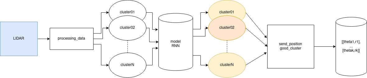
A ROS node, detector_node, subscribes to /scan. Incoming scans are clustered and converted into sequences, which are classified by the trained LSTM. Detected positions are published to /radar.
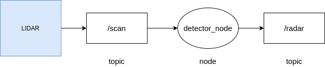
The Fig. 4 outlines the flow from scan to detections.
Clustering runs inside the subscriber callback so that raw LiDAR data are transformed into sequences before inference.
The Fig. 5 details the conversion from scan points to LSTM-ready sequences. For each positive cluster, the center computation above provides the estimated position.