Overview
The Dynamic Window Approach (DWA) is a reactive motion planning method used in mobile robotics. At each control cycle, it samples admissible velocity pairs $(v, \omega)$ and evaluates them using an objective function, selecting the pair with the highest score.
The original method presents two main issues:
- Discrete sampling, which limits precision
- High computational cost in evaluation loops
These limitations can be addressed by defining a convex, differentiable objective function and applying gradient descent for continuous optimization.
This work was presented at IEEJ SAMCON 2022, GradientPousseur 2021 .
From Sampling to Continuous Optimization
Convex Cost Function
Instead of scoring discrete samples, the cost is defined as:
$$ \mathcal{L}(v, \omega) = \lambda_1 \cdot \mathcal{C}_{goal} + \lambda_2 \cdot \mathcal{C}_{distance} + \lambda_3 \cdot \mathcal{C}_{speed} \quad \text{Eq (1)} $$
Where:
- $\mathcal{C}_{\text{goal}}$: cost for deviation from target direction
- $\mathcal{C}_{distance}$: angular penalty for proximity to obstacles
- $\mathcal{C}_{speed}$: penalty for low forward velocity
All terms are convex and differentiable, enabling gradient-based optimization.
Goal Alignment Term
The target point is obtained from a high-level controller (e.g., visual servoing). The quadratic distance between predicted and target positions is used:
$$ \mathcal{C}_{goal} = (x_{pred} - x_{target})^2 + (y_{pred} - y_{target})^2 \quad \text{Eq (2)} $$
This term encourages convergence to the desired trajectory.
Obstacle Distance Term
LiDAR data is processed to extract safe angular zones. The closest safe direction $\theta^*_{\text{final}}$ to the robot’s current heading is identified.
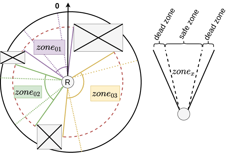
The cost penalizes deviation from this safe orientation:
$$ \mathcal{C}_{distance} = \frac{1}{2} \left( \omega - \frac{\theta^*_{\text{final}}}{dt} \right)^2 \quad \text{Eq (3)} $$
Where:
- $\omega$: angular velocity
- $\theta^*_{\text{final}}$: optimal safe angle
- $dt$: control time horizon
This method provides obstacle avoidance, similar in principle to Vector Field Histogram strategies.
Speed Regularization Term
A penalty on low velocities maintains motion:
$$ \mathcal{C}_{speed} = (v_{max} - v)^2 \quad \text{Eq (4)} $$
This prevents the robot to be stuck. Without the component, in some situations, the best solution should to stop the robot.
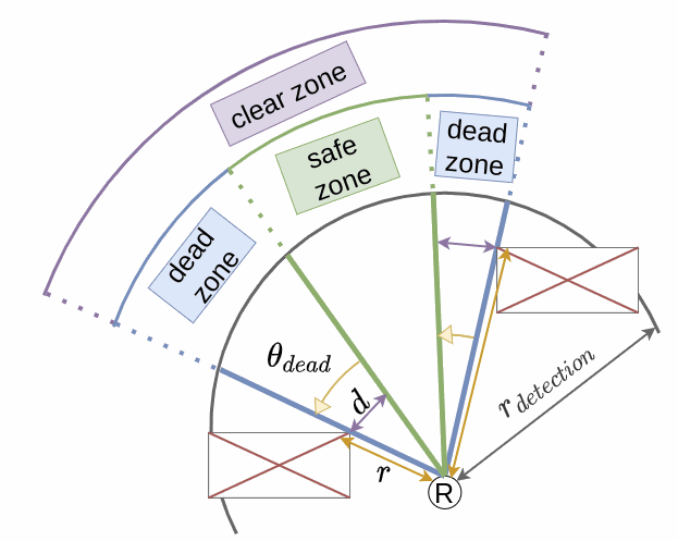
Gradient Descent Optimization
Descent Limitation
In the initial strategy, it is important to limit the values accessible to the robot. It is important to remember that the strategy must provide a solution that can be applied by the robot within a time interval $dt$. Consequently, acceleration and deceleration are taken into account, in addition to the current velocity.
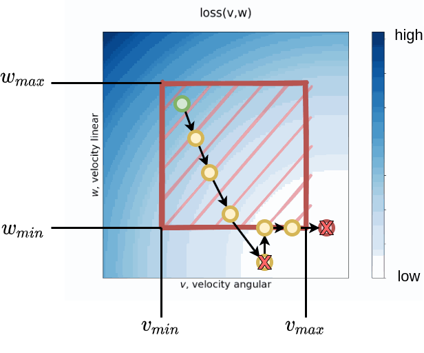
The Fig. 2 illustrates the DWA window concept combined with the gradient descent approach. The idea is to treat the window as a constraint: if the gradient descent reaches the boundary, the descent is redirected along the axis of that boundary.
Descent Formulation
The optimal control is:
$$ (v^*, \omega^*) = \arg\min_{v, \omega} \mathcal{L}(v, \omega) \quad \text{Eq (5)} $$
Gradient descent updates are applied as:
$$ \begin{bmatrix} v \\ \omega \end{bmatrix} \leftarrow \begin{bmatrix} v \\ \omega \end{bmatrix} - \eta \cdot \nabla \mathcal{L}(v, \omega) \quad \text{Eq (6)} $$
Where $\eta$ is the learning rate.
This continuous approach avoids discretization limits and improves convergence precision.
Integration with Visual Servoing
In SCANeR experiments, the optimizer was integrated with a visual servoing module that extracts a centerline from camera input. The $\mathcal{C}_{goal}$ term uses this visual reference as the target, ensuring alignment with detected lanes.
Simulation and Real Tests
Gazebo Simulation
Tested with static obstacles and known goals.
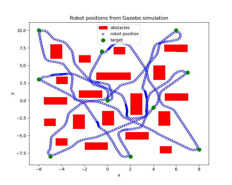
The Fig. 3 shows the path of the robot after applying the DWA optimization approch. In this test, the robot has to reach position over an unknown map.
Demo: Video 1: Video demo (Gazebo simulation) .
Turtlebot Experiments
Validated on real robots in indoor scenarios.
Demo: Video 2: Video demo turtlebot (case 1). , Video 3: Video demo turtlebot (case 2). .
This demonstration uses also this DWA optimization.
SCANeR Scenarios
Evaluated in autonomous driving simulations:
- Lane center extracted from camera images
- Optimizer computed $(v, \omega)$ toward the visual target
- Demonstrated robustness to perception noise
Demo: Video 4: Video demo (SCANeR + visual servoing). .
References
- Gradient descent dynamic window approach to the mobile robot autonomous navigation.
Hugo POUSSEUR, Alessandro VICTORINO
[Access PDF]