Motivation
As part of an autonomous driving project, I contributed to the development of a system enabling a vehicle to adapt its behavior to traffic lights. The vehicle adjusts its speed according to the current traffic light state.
The project is divided into four main components:
- Matching: Identifying traffic light positions on the map
- Detection: Determining the current state of the traffic light
- Planning: Adjusting vehicle speed according to the detection result
- Control: Applying the computed velocity to the vehicle
The detection pipeline is implemented in Python, while control is handled in C++ within a ROS2 environment.
Matching
Based on the vehicle’s planned trajectory, map elements such as traffic lights are projected onto the path.
This step does not determine the state of the lights, but flags that a traffic light zone is ahead.
Detection
Within a traffic light zone, the system must identify the current state of the light.
YOLO is used for detection. By default, YOLO is not trained to recognize traffic light states; it detects only the presence of a light. A custom YOLO model was therefore trained using a dedicated dataset for this application.
Dataset
Cameras
Multiple recording sessions were conducted using three different cameras under varying weather conditions (rain and sun) to ensure diversity.
This also enabled evaluation of the most suitable camera for detection. Key constraints included:
- Field of view
- Image contrast, even in direct sunlight
- Ease of mounting and adjustment
Labels
The dataset was annotated with the following labels:
TL_TOP_RED: 0TL_BOTTOM_RED: 1TL_TOP_GREEN: 2TL_BOTTOM_GREEN: 3TL_TOP_ORANGE: 4TL_BOTTOM_ORANGE: 5
This allows the model to distinguish both the position (top or bottom) and the color of the lights.
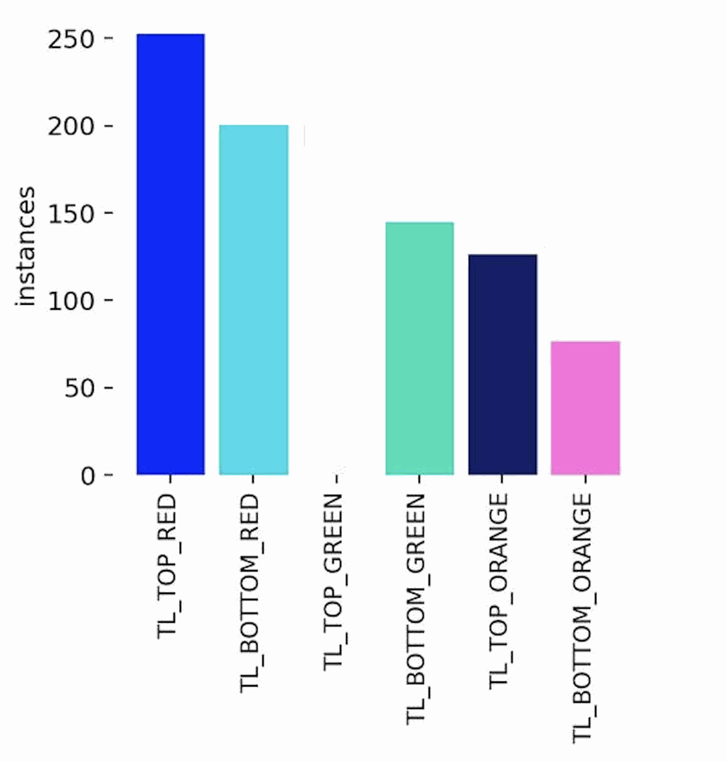
The following figure shows dataset distribution. The minimum number of samples per class was targeted. Red lights occur more often due to their longer duration.
Camera position also affects distribution: bottom lights are often obscured by trees when far away.
Training
The YOLO model was trained on this dataset.
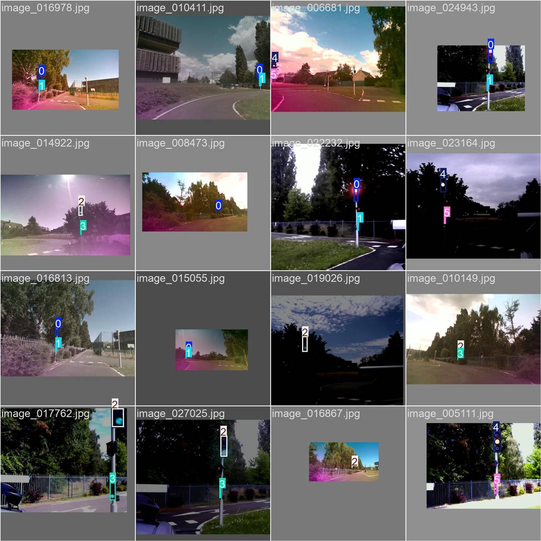
Image quality and contrast vary due to different camera sources and YOLO configurations.
Data augmentation included transformations, translations, and color adjustments to improve generalization.
After 500 epochs, the following evaluation results were obtained on the validation set:
- Precision$$ \text{Precision} = \frac{TP}{TP + FP} \quad \text{Eq (1)} $$
Measures how often the model’s positive detections (e.g., “green top light detected”) are correct.
A precision close to 1.0 means very few false positives, the system rarely claims a light is green/red/orange when it is not.
Result: ≈ 0.99 . Almost every detection made by the system is correct.
- Recall$$ \text{Recall} = \frac{TP}{TP + FN} \quad \text{Eq (2)} $$
Measures how many of the actual lights present were detected by the model.
A high recall means the model rarely misses a relevant light (false negatives are rare).
Result: ≈ 0.97 . The system detects almost all visible traffic lights.
- mAP@0.5$$ \text{mAP@0.5} = \text{mean}(AP_{\text{IoU}=0.5}) \quad \text{Eq (3)} $$
Mean Average Precision across all classes, calculated at an IoU (Intersection-over-Union) threshold of 0.5.
IoU is the overlap ratio between the predicted bounding box and the ground-truth box.
A value near 1.0 means the predicted box is well-aligned with the real light location.
Result: ≈ 0.98 . Bounding boxes are accurate for most detections.
- mAP@[0.5:0.95]$$ \text{mAP}_{[0.5:0.95]} = \frac{1}{10} \sum_{i=0}^{9} AP_{0.5 + 0.05i} \quad \text{Eq (4)} $$
Average precision computed over multiple IoU thresholds from 0.5 to 0.95 in steps of 0.05.
This is a stricter metric than mAP@0.5 because it requires good alignment across a range of IoU tolerances.
Result: ≈ 0.83 . Performance remains high even under stricter bounding box alignment requirements.
- F1-score$$ F1 = 2 \cdot \frac{\text{Precision} \cdot \text{Recall}}{\text{Precision} + \text{Recall}} \quad \text{Eq (5)} $$
The harmonic mean of precision and recall, a balanced single score that considers both false positives and false negatives.
Result: ≈ 0.98 . The detector maintains a strong balance between correctly identifying lights and not missing them.
These results confirm the detector is both accurate (high precision) and comprehensive (high recall), with bounding boxes that closely match ground truth (high mAP).
This reliability is crucial for control decisions, since a missed red light or a false green could lead to unsafe vehicle behavior.
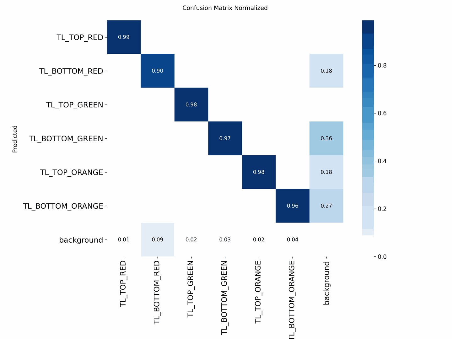
| Class | Accuracy | Notes |
|---|---|---|
| TL_TOP_GREEN | ≈ 0.98 | Minor confusion with background and BOTTOM_GREEN |
| TL_TOP_RED | ≈ 0.99 | Nearly perfect detection |
| TL_BOTTOM_RED | ≈ 0.90 | Some confusion with background |
| TL_BOTTOM_GREEN | ≈ 0.97 | Confused with TL_BOTTOM_ORANGE |
| TL_TOP_ORANGE | ≈ 0.98 | Minor confusion with BOTTOM_ORANGE and background |
| TL_BOTTOM_ORANGE | ≈ 0.96 | Confused with TL_BOTTOM_GREEN |
Examples
Examples of detection on real-world data are shown below.
Current implementation focuses on top lights, as bottom lights are not always visible.
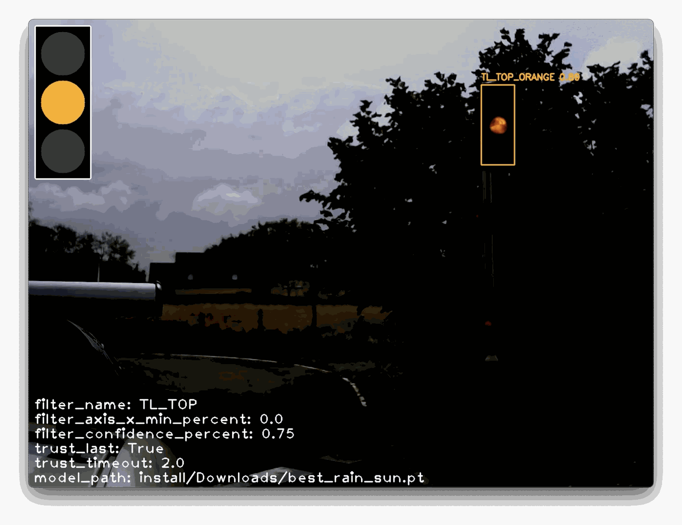
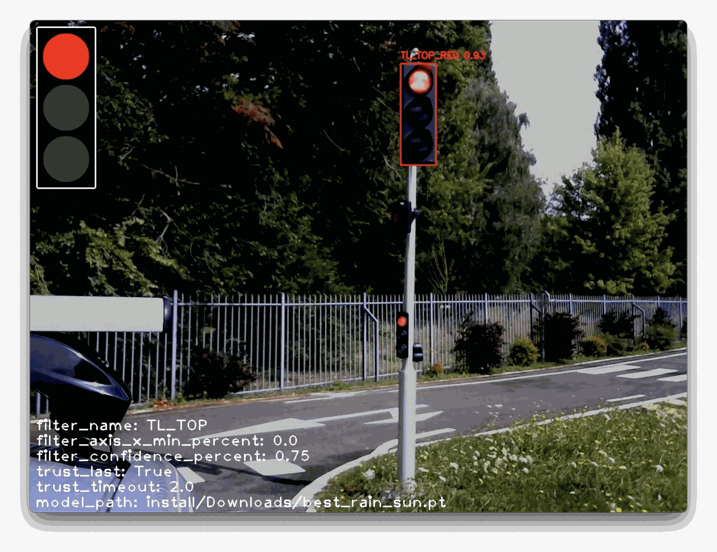
The drawn traffic light overlay represents the system’s recognized state.
ROS Integration
Pipeline
The pipeline is divided into four parts:
detection_rate: Adjusts the detection rate of the pipeline by modulating the publishing frequency of the input image, effectively reducing the initial processing rate;detection_detect: Detects the bounding boxes (bbox) of the TOP_ and BOTTOM_ elements in the image;detection_filter: Applies filtering on the detections, for example by name (e.g., excluding BOTTOM elements), by X-position, or by confidence score;detection_state: Determines the current traffic light state based on the filtered detections.
State Deduction and Propagation
The map is used to identify traffic lights along the planned route.
The detection_state node publishes the deduced state of each detected traffic light.
By default, the state is determined as follows:
- If TOP_ is detected with sufficient confidence → STATE = COLOR VALUE from TOP_{RED, ORANGE, GREEN} class;
- If TOP_ is not detected with good confidence but BOTTOM_ is → STATE = COLOR VALUE BOTTOM_{RED, ORANGE, GREEN} class;
- If neither TOP_ nor BOTTOM_ provides a reliable classification → STATE = NOT DETECTED
The node includes a timeout parameter that preserves the last valid detection when no new result is produced, preventing sudden or unwarranted braking.
If no detection is available after the timeout, the state becomes not detected, in which case the decision server applies the same precautionary strategy as if the light were red.
The detection node runs at 10 Hz, providing a balance between computational cost and system responsiveness. Given the deterministic nature of the model and the camera’s 30 Hz frame rate, increasing the inference rate offers no practical benefit.
Adaptive Control
Once the traffic light state is determined, the vehicle’s speed profile is adjusted accordingly.
Each road element (including each traffic light) is associated with a finite state machine defining vehicle behavior. A speed profile is assigned based on distance, for example:
$ d \in [0, distance_{ahead}],\ speed = profile(d)$.
The traffic light state machine is defined as:
LOCK: Element is active; vehicle stops before the lightSKIP: Element is ignored; vehicle continuesFREE: Element passed; no longer relevant, handler manager can remove the traffic light handler
Transitions:
LOCK$\Longleftrightarrow$SKIPSKIP$\Longrightarrow$FREE
State updates based on detected light color:
LOCK: red or orange (depending of the reach time)SKIP: greenFREE: light already passed
The final control signal is computed by combining all velocity profiles (traffic light state + stop state + obstacles + …) and taking the minimum value at each distance point, ensuring compliance with all constraints.
Smooth Break:
To avoid abrupt braking when the traffic light changes from GREEN to ORANGE, the time required to reach the traffic light is computed by defining the relative distance to the traffic light and considering the vehicle’s current speed.
Based on this time, the decision logic chooses between switching the state to LOCK (stop) or keeping the SKIP state.
$$ time_{reach} = \frac{distance_{relative}}{|speed_{vehicle}| + \epsilon} \quad \text{Eq (6)} $$
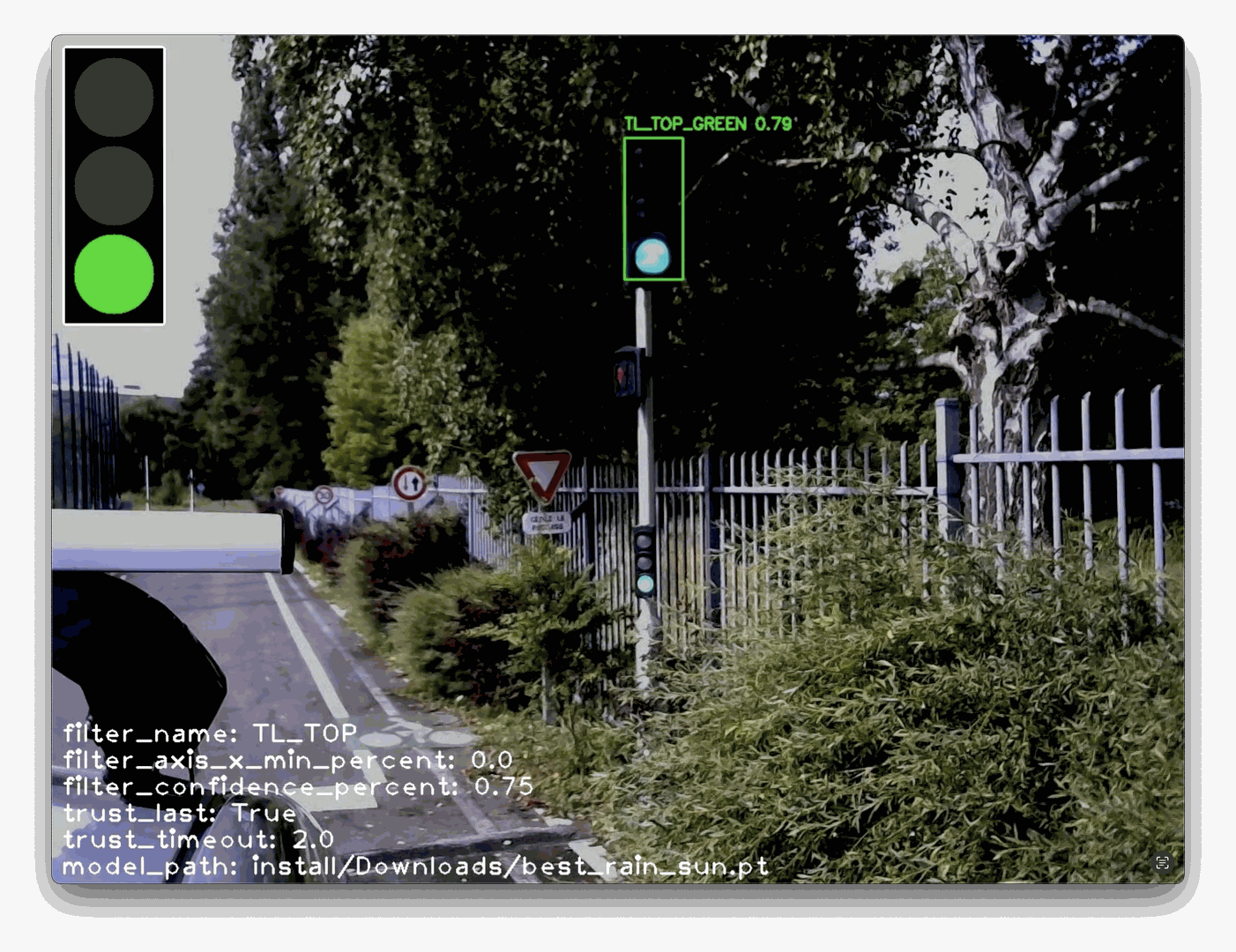
RQT
Rqt integration displaying the current traffic light state as perceived by the pipeline and the image annoted. It’s possible to use RQT and then combined rqt_image_view + image state widget, but finnaly the rqt_image_view plugin it’s to unstable, and often necessite to reload the topic, to see the image.
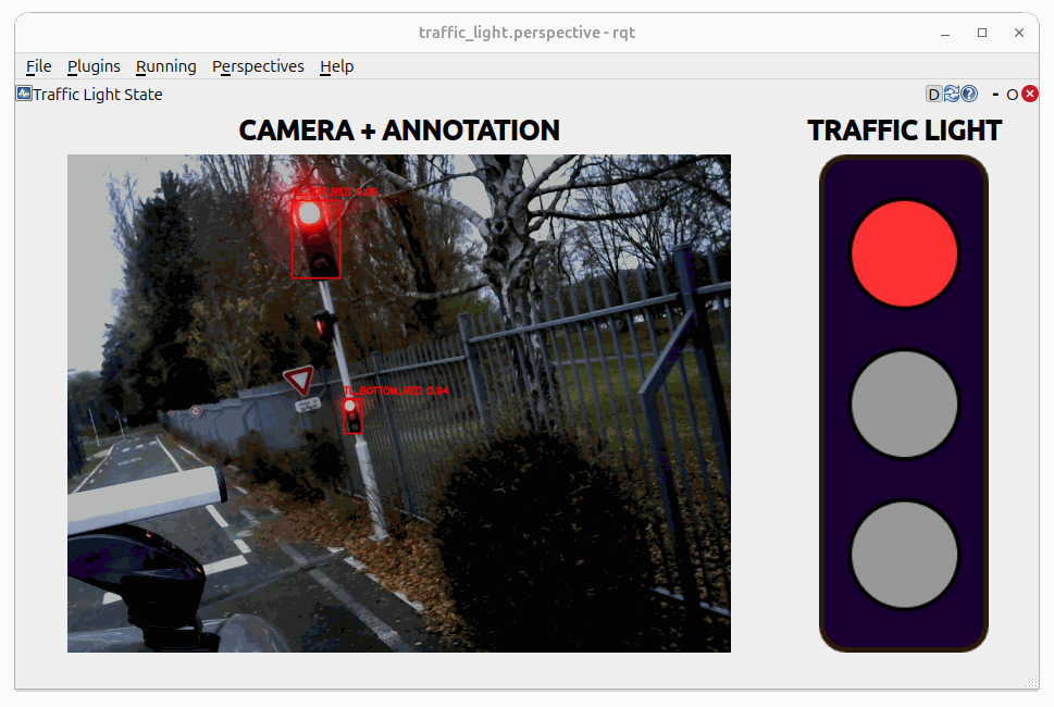
The Fig. 5 shows a screenshot of the Traffic Light State in RQT. On the left is the image annotated with the position and classification estimates, and on the right is the pipeline’s resulting deduction based on those classification outputs.