Demonstration
Overview
As part of a collaborative autonomous driving project, I contributed to the implementation of the core planning functionalities for autonomous driving.
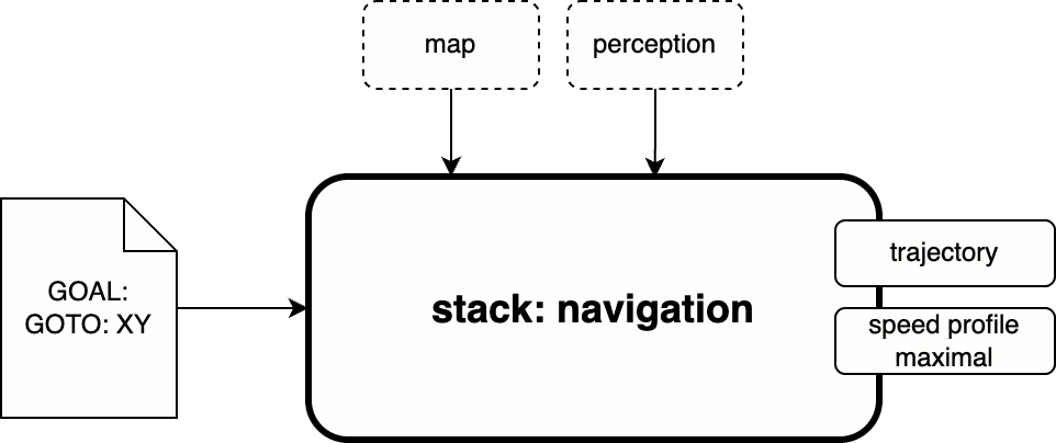
The navigation stack transforms a target position into a safe and efficient motion trajectory using environmental context and map information.
The process is divided into three stages:
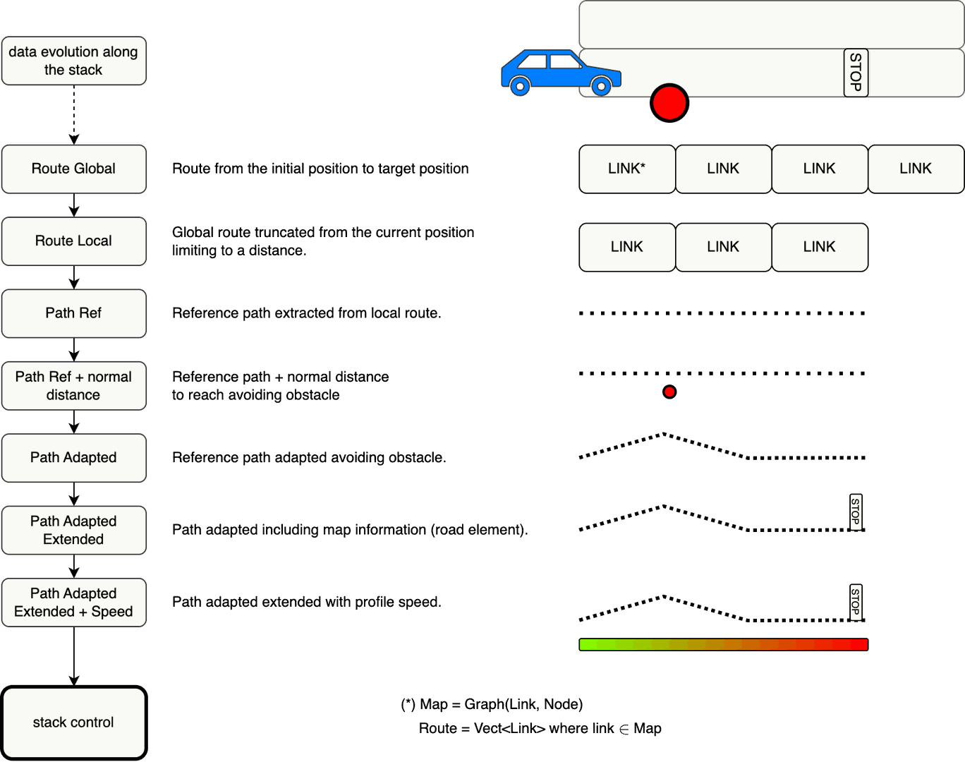
- Global route computation: finding a feasible route on the road network
- Local path generation: adjusting the trajectory to avoid obstacles
- Motion profile optimization: generating smooth and feasible velocities along the path
Navigation Stack Architecture
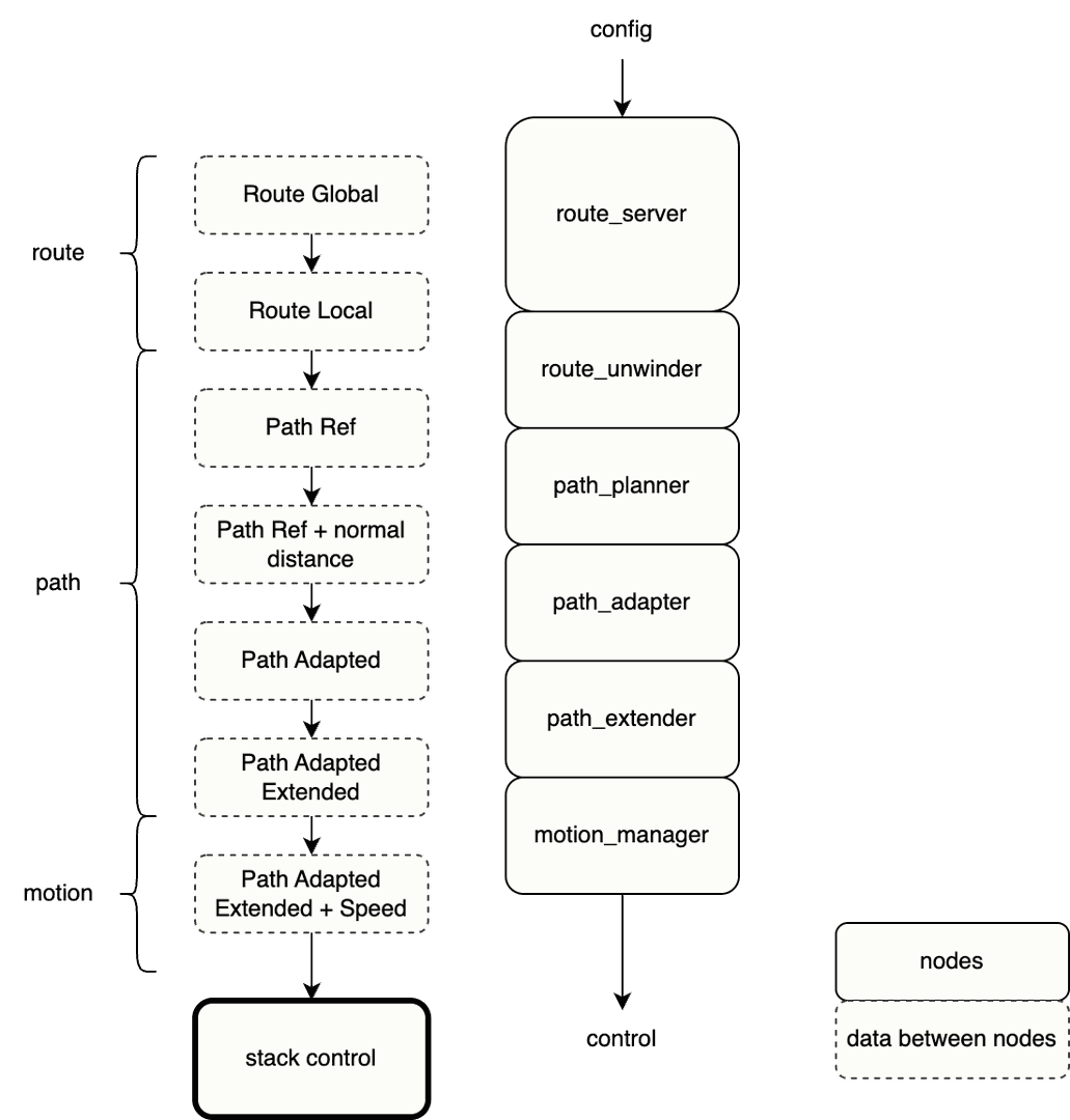
The architecture follows a modular structure in ROS2. Each node is responsible for a specific step in the planning pipeline:
- Route Server: computes the topological path
- Path Planner + Path Adapter: modifies the route to avoid obstacles
- Motion Manager: assigns a feasible velocity profile
- Controller: executes the commands
Global Route Planning
Responsibilities
The Route Server node computes the route from the current vehicle position $A$ to the goal $B$, using algorithms such as Dijkstra or A*. The process includes:
- Matching the vehicle’s current position on the HD map
- Matching the target goal
- Planning the shortest or safest path $\mathcal{P}(A, B)$
- Providing a ROS2 service to compute routes for a queue of goals ${B_1, B_2, \dots}$
Integrated Planning Stack
Closed-loop autonomous operation is achieved by chaining:
- Target reception → global route
- Obstacle analysis → adjusted path
- Velocity assignment → dynamic feasibility
- ROS2 interface → command execution
Path Planning
Problem
Even when a global route exists, dynamic obstacles may obstruct the reference trajectory. A local path must be adapted in real time to maintain safety.
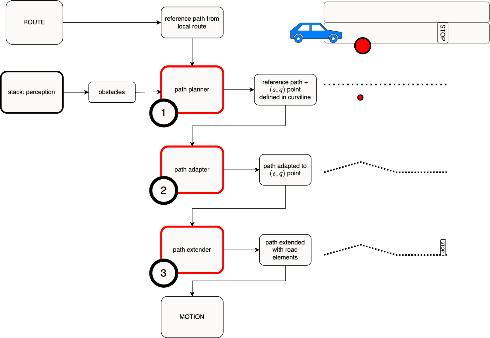
Local Path Planner
This module scans the global path to determine whether obstacles intersect it. When an obstacle is detected, the system computes:
- The longitudinal distance $s$ at which the obstacle interferes
- The required lateral shift $q(s)$ needed to avoid the obstacle
The planner then outputs a new trajectory by adjusting the centerline accordingly.
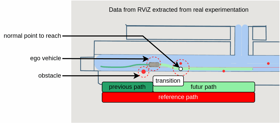
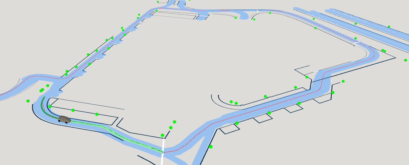
The design is based on research from LocalSaid 2023 . The animation below illustrates a Python-based simulation used to evaluate the solution and guide the design of an architecture suitable for integration into the navigation stack. The method from the original reference has been adapted to meet specific system requirements.
Interpolation
To define a smooth trajectory in the plane, the path is represented using curvilinear interpolation, where $x(d)$ and $y(d)$ are interpolated independently as functions of the arc length parameter $d$.
Cubic splines are commonly used for this purpose, ensuring continuity of position, first derivative (tangent), and second derivative (curvature). The path is thus defined by:
$$ \gamma(d) = \begin{pmatrix} x(d) \\ y(d) \end{pmatrix} \quad \text{Eq (1)} $$
Where:
- $d$: curvilinear abscissa (arc length) along the path
- $x(d)$, $y(d)$: smooth spline interpolations based on reference waypoints
This approach enables the evaluation of geometric quantities such as direction and curvature at any point along the trajectory.
Motion Profile Generation
The speed profile of a vehicle depends on various factors, including:
- Road elements (e.g., stop signs, traffic lights, speed bumps)
- Obstacles on the road (e.g., vehicles, pedestrians)
Speed Profile: Signal
To combine these different inputs, a speed signal profile is used. This is represented as a step signal indicating the maximum allowed speed at each point along the trajectory (x-axis: distance, y-axis: maximum speed).
This representation is efficient because only the key change points are defined, with the speed assumed constant between two points.
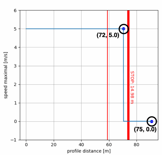
Example:
distance [m]:    72.0  | 75.0
speed [m/s] :     5.0  |  0.0
This specifies a speed of 5.0 m/s until 75.0 meters, where it drops to 0.0 m/s.
Speed Profile: Road Element Handler
Each road element is associated with a handler.
The purpose of the handler is to define the Finite State Machine (FSM) of that element.
Each state of the element specifies a corresponding speed signal.
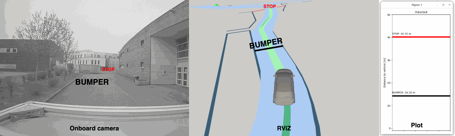
Example: STOP
A STOP road element, exploits the handler HandlerLockWait
A HandlerLockWait element defines three states:
| State | Description | Signal |
|---|---|---|
| LOCK | The stop is active. The signal remains UP until the vehicle reaches the stop, then becomes 0. | UP → 0 |
| WAIT | The vehicle has reached the stop and is waiting for permission to start. | 0 |
| FREE | The vehicle has passed the stop. | UP |
State Transitions
Automatic Transitions
Some transitions occur automatically. In these case the state machine can apply the transition himself, without autorisation.
For example:
LOCK → WAITThis happens once the vehicle reaches the stop position and its speed equals 0. The vehicle performs this transition autonomously.
Permission-Based Transitions
Other transitions require explicit permission. In these case the state machine should wait a permission (a flag), to inform the transition is possible.
For example:
WAIT → FREEThis transition requires authorization from the decision server, ensuring the decision layer has confirmed it is safe for the vehicle to proceed.
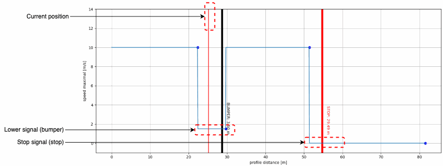
Speed Profile: Combined Signals
Multiple signals can be combined by taking the minimum at each point, ensuring compliance with all constraints.
The example below shows two road elements: a speed bump and a stop sign.
- The speed bump requires slowing to approximately $ v \approx 1.8\ \text{m/s} $.
- The stop sign requires a complete stop ($ v = 0\ \text{m/s} $).
Speed Profile: Curvatures
Speed Profile: Demonstration
References
- Local trajectory planning for autonomous vehicle with static and dynamic obstacles avoidance
Abdallah Said, Reine Talj, Clovis Francis, Hassan Shraim
IEEE ITSC 2021
[Access PDF]