Demonstration
Info: A video demonstration of the decision-making system is coming soon.
Introduction
In autonomous driving, the vehicle must be able to make a series of decisions, such as slowing down, stopping at an intersection, or waiting until the road is clear before proceeding.
These decisions depend on the behavior of other road users. The system must therefore identify surrounding obstacles and determine which ones are relevant for decision-making.
We define two complementary approaches:
- Perception: performed using a LiDAR sensor, providing a precise 3D view of the environment.
- Critical zone: a map-based region that defines where the vehicle should pay special attention to obstacles, depending on the situation.
Disclaimer: This stack was initially developed in Python as a proof of concept (PoC). Once validated, it will be reimplemented in C++ to improve performance and execution speed.
Critical Zone
In situations such as approaching a stop sign, yielding, or crossing an uncontrolled intersection, the vehicle must decide whether to proceed or wait.
This decision depends on the presence of other vehicles or obstacles within a specific area of interest called the critical zone.
The process is divided into two steps:
- Using the vehicle’s map + Road Rules, identify the lanes necessary to a decision, this defines the critical zone.
- Focus perception and filtering on this zone to determine if it is empty or occupied.
The decision logic is binary:
- if the critical zone is empty, the vehicle can proceed.
- if it is occupied, the vehicle must wait or slow down.
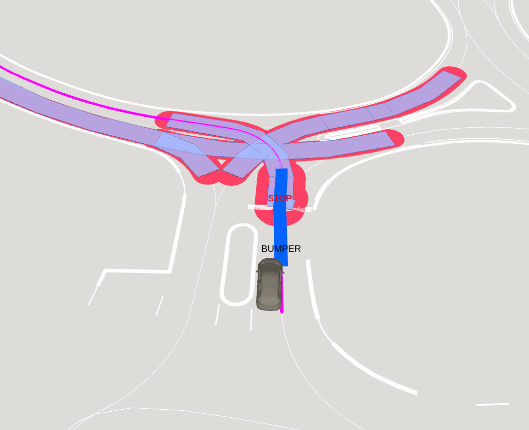
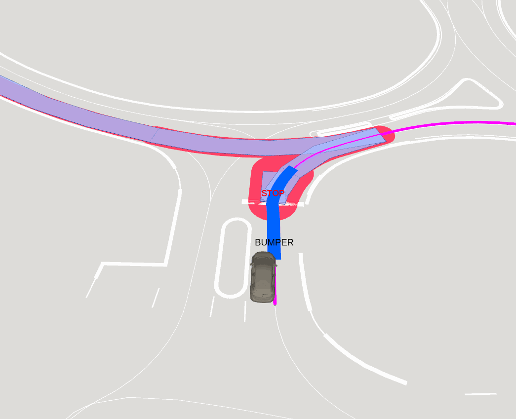
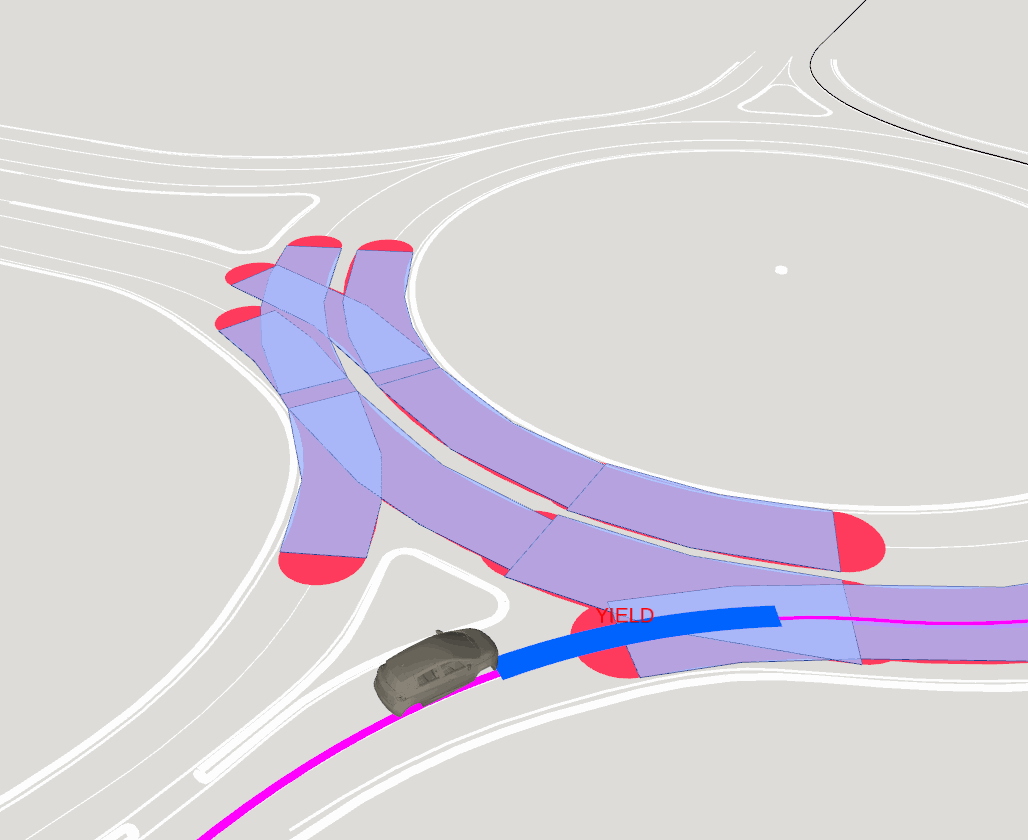
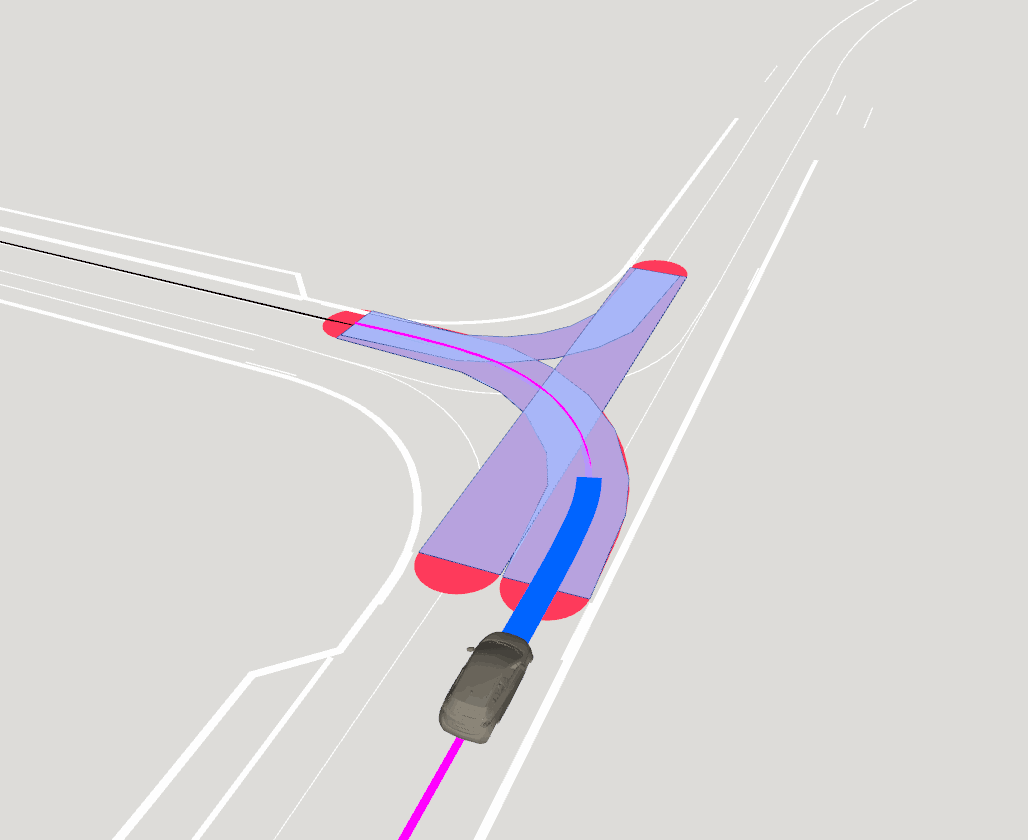
The Fig. 1 and Fig. 2 illustrate how the critical zone adapts depending on the path geometry and the road rules. In practice, the critical zone must adapt to the right-of-way rules and the type of road element (e.g., stop sign, intersection, roundabout). This prevents defining an overly strict critical zone that would unnecessarily block the vehicle’s progress.
Legend:
- Red lines: represent critical zone lines from the map;
- Blue polygones: represent polygones from the critical zone lines, used for filtering;
Detection
The perception stack relies on a geometric LiDAR-based approach.
Unlike deep-learning methods, this pipeline is deterministic and explainable, every detection can be interpreted and justified.
Starting from a raw LiDAR point cloud (PCL2), the system identifies a set of obstacles (Perceptions[]) represented by ground-projected polygons.
These obstacles can influence the vehicle’s motion when:
- An object lies on the planned driving path;
- An object is within a defined critical zone.
Note: The adaptive control is performed by the perception + the signal obstacle created by the motion manger
Pipeline
To filter obstacles along the path or within critical zones, the pipeline generates Perceptions[] objects aligned with the map frame.
From these, filtered subsets are computed depending on the driving context.
Main
| Step | I/O : type (frameid) | Description |
|---|---|---|
| 1. Point Filtering | PCL2 (lidar) → PCL2 (lidar) | Filters raw LiDAR points by height (z_min, z_max) and range limits to remove ground or distant noise. |
| 2. Voxel Downsampling | PCL2 (lidar) → PCL2 (lidar) | Reduces cloud density using voxel grid filtering for faster processing. |
| 3. Clustering (Voxel-based) | PCL2 (lidar) → PCL2 (lidar) | Groups nearby points using voxel-based connected components in 2D/3D space, efficient and stable segmentation. |
| 4. Cluster Filtering | PCL2 (lidar) → PCL2 (lidar) | Removes clusters below size or height thresholds to discard irrelevant objects. |
| 5. TF Transform (Clusters) | PCL2 (lidar) → PCL2 (map) | Transforms clustered points to the map frame for spatial consistency. |
| 6. Road Polygon Filtering | PCL2 (map) → PCL2 (map) | Keeps only clusters overlapping with the road polygons from the map. |
| 7. Cluster → Perceptions | PCL2 (map) → Perceptions[] (map) | Converts clusters into perception objects with bounding boxes and 2D footprints. |
| 8. Perception Filtering | Perceptions[] (map) → Perceptions[] (map) | Filters perceptions by area or geometry constraints to retain valid obstacles. |
Main + On Path
| Step | I/O type (frameid) | Description |
|---|---|---|
| 9. Path → Polygons (Local) | Path (map) → Polygons[] (map) | Generates polygons around the navigation path for footprint validation and filtering. |
| 10. Perceptions on Path Filter | Perceptions[] (map) + Polygons[] (map) → Perceptions[] (map) | Keeps only perceptions intersecting the drivable corridor, focusing on relevant obstacles. |
Main + On Critical Zone
| Step | I/O type (frameid) | Description |
|---|---|---|
| 9. Critical Zone Polygons | Map (map) → Polygons[] (map) | Converts the map-defined critical zone into polygons used for decision-making. |
| 10. Perceptions in Critical Zone Filter | Perceptions[] (map) + Polygons[] (map) → Perceptions[] (map) | Keeps only perceptions located inside critical zones for safety evaluation. |
Cluster To Perception
The step 7. Cluster → Perceptions represents the transformation from clustered PointCloud2 data, meaning the point cloud includes a cluster ID channel, into an array of Perception objects.
Each Perception defines the shape and footprint of an obstacle. The footprint is represented by a polygon.
Footprint Polygons Steps:
- Make a grid: Create a blank image that covers all the points.
- Plot the points: Mark each point as a white pixel on the grid.
- Morphological closing: Use dilation + erosion to connect nearby points and fill small gaps.
- Smooth: Optionally blur the image to make shapes more rounded.
- Threshold + dilate: Convert back to binary and slightly thicken shapes.
- Find contours: Detect continuous white regions (these become polygon boundaries).
- Convert back to real coordinates: Map pixel positions to the original coordinate system.
- Clean polygons: Use Shapely to fix invalid shapes, remove very small ones, and handle multiple regions.
- Return polygons: Output valid Shapely polygons representing the connected areas of points.
Example on Real Data
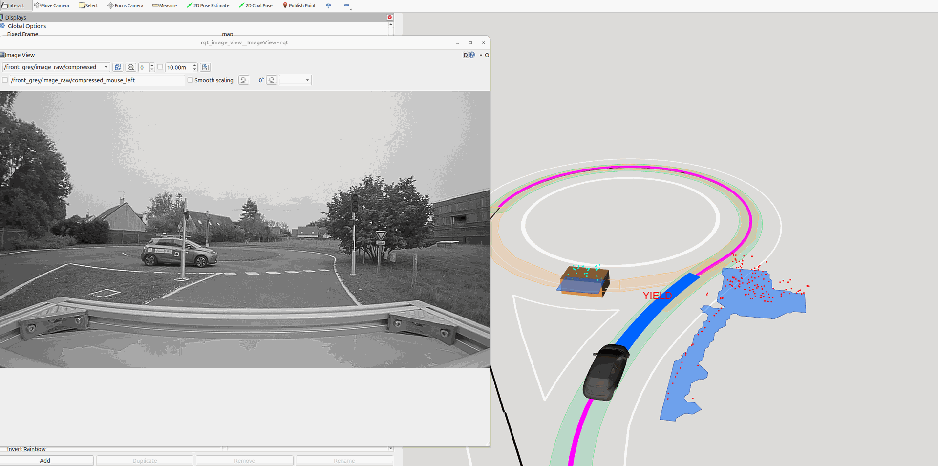
The
Fig. 3
illustrates a real-data example.
On the left is the camera image showing the driving situation. Note that the camera is not used for detection.
On the right, the RViz visualization displays the LiDAR-based perception results.
Legend:
- Green lane: Polygon of the planned path the vehicle will follow.
- Orange lane: Polygon representing the critical zone.
- Red dots + blue polygon (right): A cluster detected by the pipeline, close to the map area but ignored after path and critical-zone filtering.
- Green dots + orange shape + blue polygon: The detected vehicle obstacle located within >the critical zone. The orange overlay indicates that this object lies inside the critical zone.
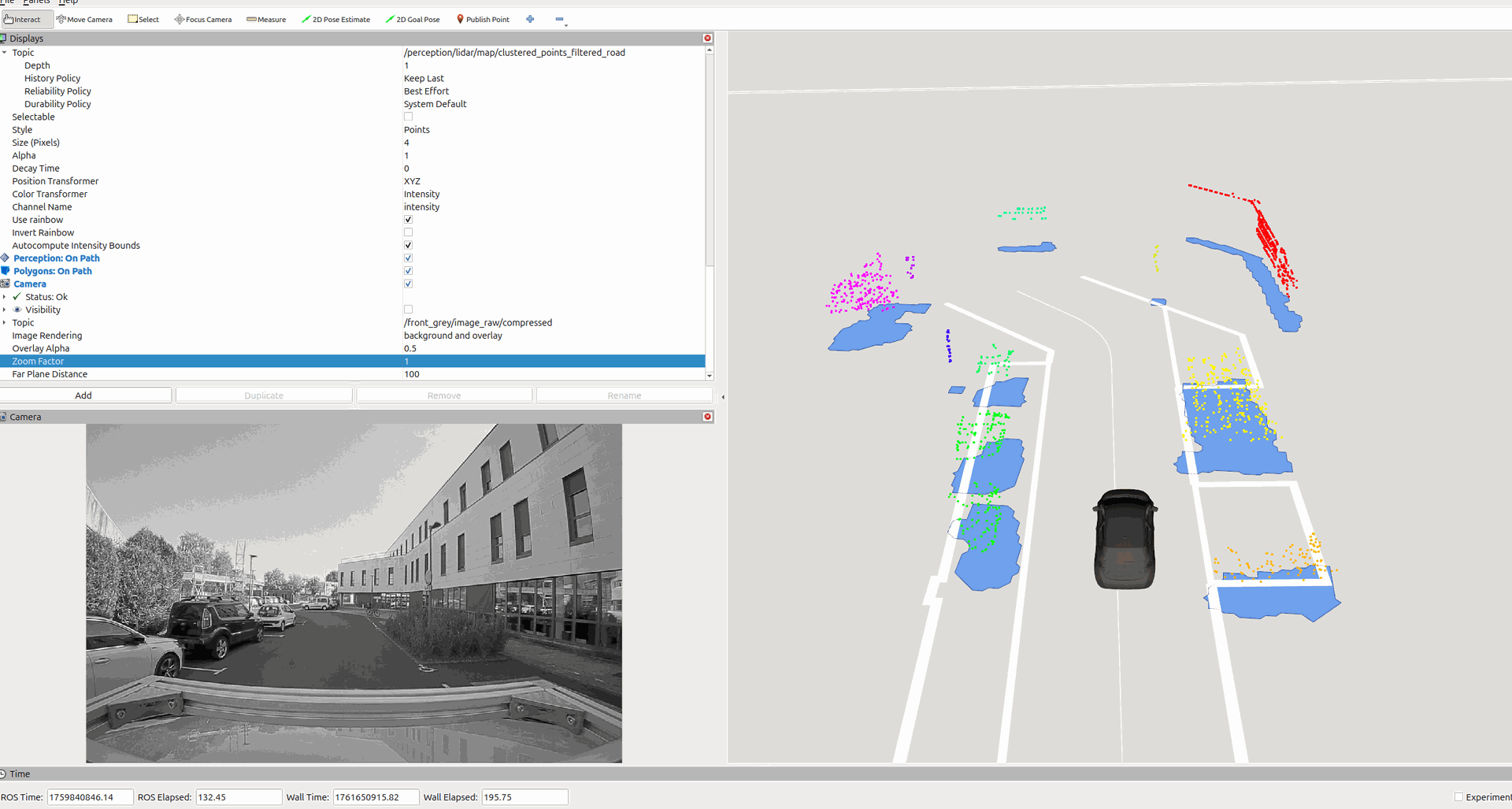
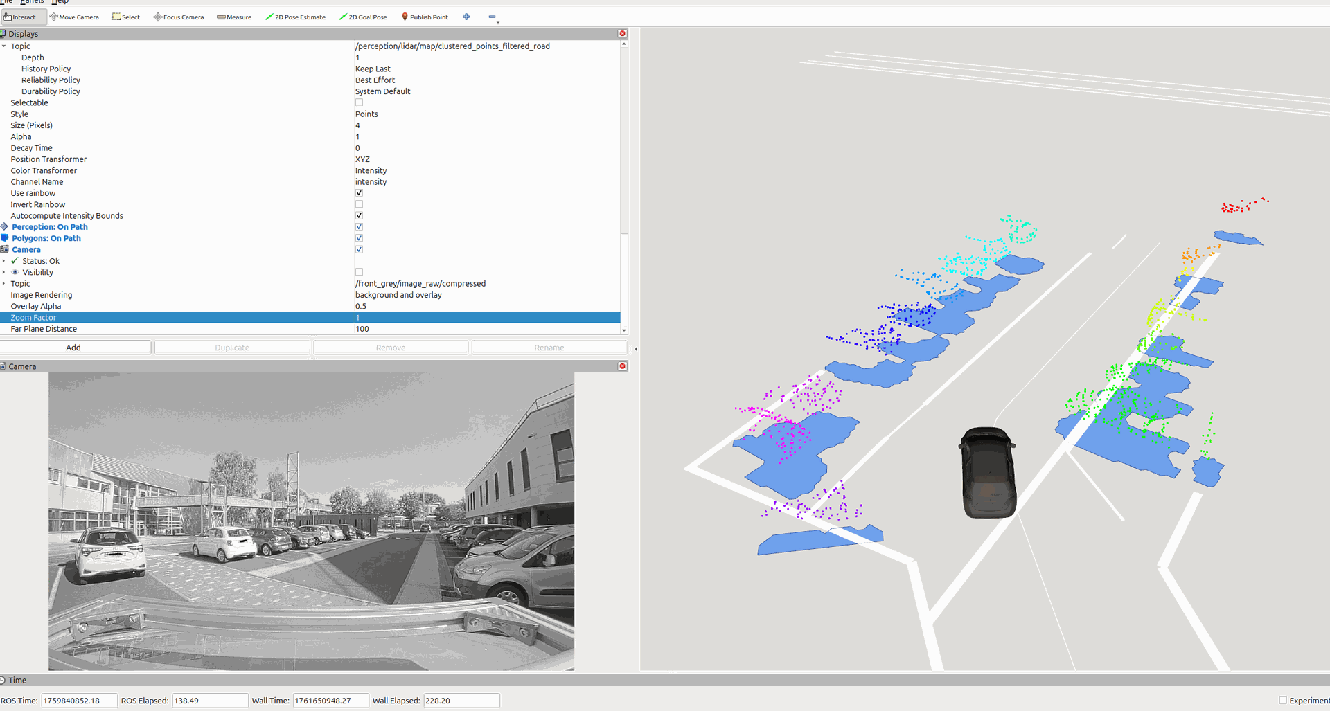
The Fig. 4 , Fig. 5 show different detections examples in different situations.
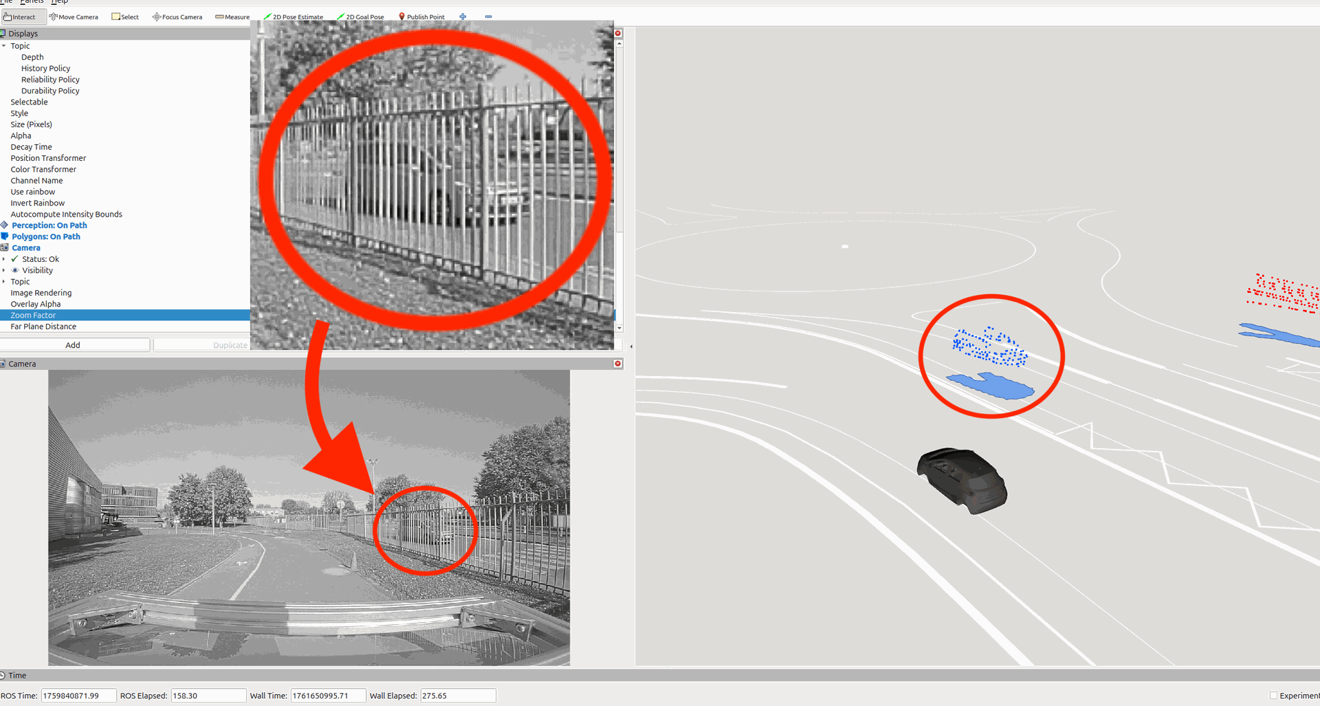
The Fig. 6 shows an example where the pipeline detection can detect a vehicle through the barrier between the ego vehicle and the vehicle detected. The red circle shows the vehicle in the image frame and RViZ display.