Demonstration
Overview
As part of a collaborative autonomous driving project, I contributed to the low-level control system responsible for translating navigation commands into actuator signals (steering and torque).
This system is fully integrated into a ROS2-based autonomous stack and has been deployed and tested on a real electric vehicle with in-wheel motors.
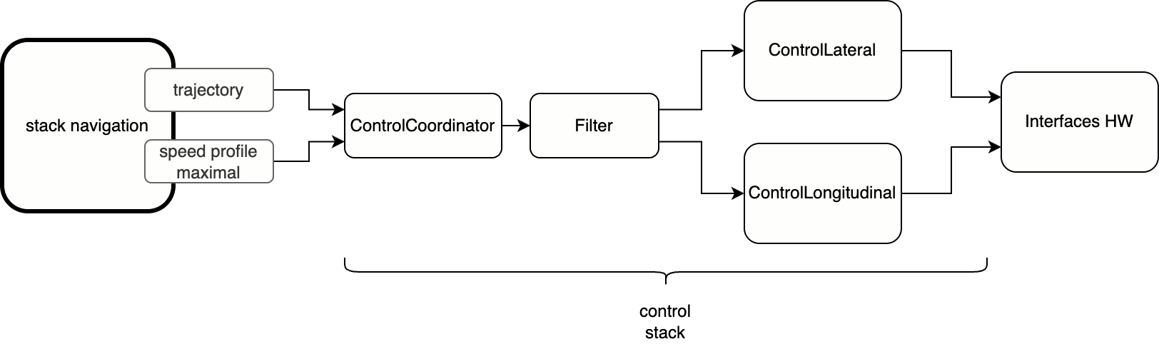
Control Structure
The controller is composed of two main components:
- Lateral control: Aligns the vehicle to a reference trajectory via steering input.
- Longitudinal control: Tracks a target speed while respecting acceleration and deceleration constraints.
Both control loops run at 100 Hz and are tuned for real-time performance on embedded systems.
Longitudinal Control
A classical PID controller is used to track the target velocity:
$$ u(t) = K_p \cdot e(t) + K_i \cdot \int_0^t e(\tau)\, d\tau + K_d \cdot \frac{de(t)}{dt} \quad \text{Eq (1)} $$
Where:
- $u(t)$: torque or throttle command
- $e(t) = v_{\text{ref}}(t) - v(t)$: velocity error
- $K_p$, $K_i$, $K_d$: proportional, integral, and derivative gains
The controller is tuned for a smooth response and fast convergence, with clamping on acceleration/deceleration to ensure passenger comfort.
Speed Profile Design
Motivation
In scenarios such as stop lines or crossing zones, it is important to smoothly reduce velocity. Sharp deceleration causes discomfort and can lead to controller overshoot. Two types of speed profiles were evaluated.
Linear Profile
A simple constant deceleration model:
$$ v(d) = v_0 - \dot{v} \cdot d \quad \text{Eq (2)} $$
Where:
- $v(d)$: target speed at distance $d$
- $v_0$: initial velocity
- $\dot{v}$: constant deceleration
Elliptical Profile
The elliptical profile models more natural, human-like deceleration behavior. It defines velocity as a function of distance to a stopping point:
$$ v(d) = v_{\text{max}} \cdot \sqrt{1 - \left( \frac{d}{d_{\text{stop}}} \right)^2} \quad \text{Eq (3)} $$
Where:
- $v(d)$: current velocity based on remaining distance $d$
- $v_{\text{max}}$: maximum speed when far from the stop point
- $d_{\text{stop}}$: total distance over which the vehicle stops
With its derivative:
$$ \frac{\partial v}{\partial d} = -\frac{v_{\text{max}} \cdot d}{d_{\text{stop}}^2 \cdot \sqrt{1 - \left( \frac{d}{d_{\text{stop}}} \right)^2}} \quad \text{Eq (4)} $$
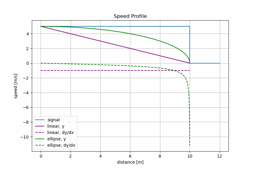
Benefits:
- Smooth, gradual deceleration at the beginning
- Sharper slowdown near the end
- More realistic than linear profiles
Profile Fusion
Curvature
Consider a planar curve $\gamma(d) = (x(d), y(d))$, parameterized by the curvilinear distance $d$.
The curve is interpolated using two independent cubic splines: one for $x(d)$ and one for $y(d)$.
The curvature $\kappa(d)$ is given by:
$$ \kappa(d) = \frac{x'(d)\, y''(d) - y'(d)\, x''(d)}{\left( x'(d)^2 + y'(d)^2 \right)^{3/2}} \quad \text{Eq (5)} $$
Where:
- $x’(d)$: first derivative of $x$ with respect to $d$
- $x’’(d)$: second derivative
- similarly for $y(d)$
Since $d$ is arc length, curvature is purely spatial and speed-invariant.
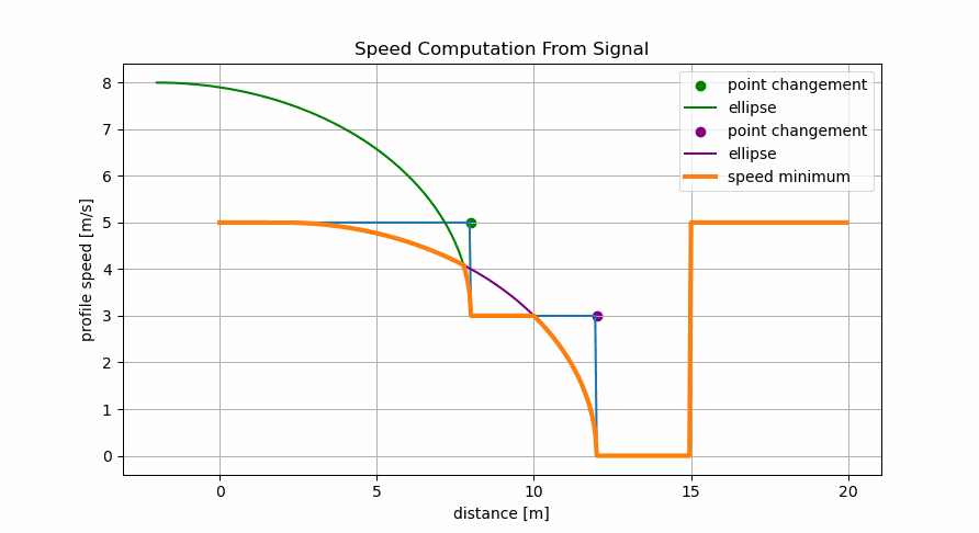
Fusion
The final velocity profile is computed by:
- Generating multiple profile candidates (e.g., obstacle, stop line, speed limit) and taking the minimal value at each point to combine them.For more details, refer to the Motion Profile Generation section of Planning Project.
- Applying an elliptical profile for deceleration scenarios.
- Taking the point-wise minimum across all profiles.
The final reference velocity includes curvature as:
$$ v_{\text{target}}(d) = \min \left( v_{\text{signal}}(d),\ v_{\text{curve}}(d),\ v_{\text{limit}} \right) \quad \text{Eq (6)} $$
Lateral Control
The lateral controller computes a steering angle to minimize both lateral offset and heading error with respect to the reference trajectory. The control law is a nonlinear feedback approach combining geometric and kinematic considerations:
$$ \theta_{\text{wheel}} = \alpha_1 \cdot \frac{L}{v^2 + D} \cdot (-e_{\text{lat}}) + \alpha_2 \cdot \frac{L}{v + D} \cdot e_{\text{heading}} + \alpha_3 \cdot L \cdot \kappa \quad \text{Eq (7)} $$
Where:
- $e_{\text{lat}}$: lateral position error
- $e_{\text{heading}}$: heading angle error
- $L$: wheelbase
- $v$: speed
- $\kappa$: path curvature
- $\alpha_1$, $\alpha_2$, $\alpha_3$: control gains
- $D$: damping constant
The steering command is then scaled:
$$ \theta_{\text{steering}} = K \cdot \theta_{\text{wheel}} \quad \text{Eq (8)} $$
Controller Properties
- Increased sensitivity to errors at low speed
- Stability across different velocity ranges
- Improved tracking in curves through curvature compensation
This controller was tested on a real electric AV, showing consistent trajectory tracking in varied scenarios.
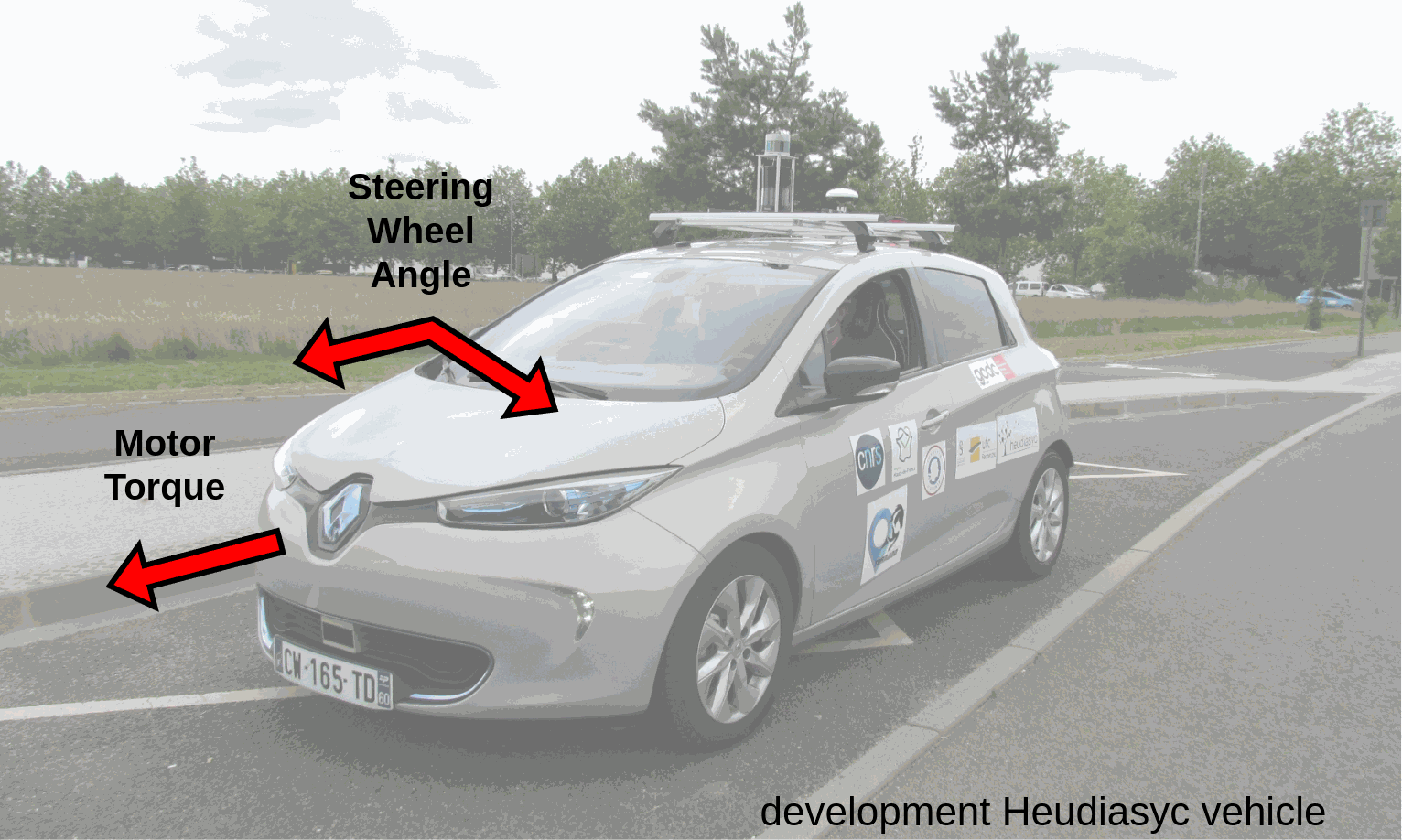
Real Vehicle Deployment
Testing was carried out on a real electric vehicle equipped with:
- RTK-GPS and IMU for high-precision localization
- A ROS2-based onboard PC running the full autonomy stack
The control system directly commanded:
- Vehicle torque
- Front steering actuator
Tested Scenarios:
- Curved roads, roundabouts, sharp and soft turns
- Straight segments with varying navigation constraints